EEG Feature Extraction Using Genetic Programming for the Classification of Mental States


1
Departamento de Ingeniería Industrial, Tecnológico Nacional de México/IT de Tijuana, Calzada Del Tecnológico S/N, Fraccionamiento Tomas Aquino, Tijuana, Baja California C.P. 22414, Mexico
2
Doctorado en Ciencias de la Ingeniería, Departamento de Ingeniería Eléctrica y Electrónica, Tecnológico Nacional de México/IT de Tijuana, Blvd. Industrial y Av. ITR Tijuana S/N, Mesa Otay, Tijuana, Baja California C.P. 22500, Mexico
3
IMB UMR CNRS 5251—CQFD Team, Bordeaux University, INRIA, 200 Av de la Vieille Tour, 33405 Talence, France
4
351 Cours de la Libération, Bordeaux University, 33405 Talence, France
*
Author to whom correspondence should be addressed.
Algorithms 2020, 13(9), 221; https://doi.org/10.3390/a13090221
Submission received: 28 July 2020
/
Revised: 28 August 2020
/
Accepted: 31 August 2020
/
Published: 3 September 2020
(This article belongs to the Special Issue Genetic Programming)
Abstract
:The design of efficient electroencephalogram (EEG) classification systems for the detection of mental states is still an open problem. Such systems can be used to provide assistance to humans in tasks where a certain level of alertness is required, like in surgery or in the operation of heavy machines, among others. In this work, we extend a previous study where a classification system is proposed using a Common Spatial Pattern (CSP) and Linear Discriminant Analysis (LDA) for the classification of two mental states, namely a relaxed and a normal state. Here, we propose an enhanced feature extraction algorithm (Augmented Feature Extraction with Genetic Programming, or FEGP) that improves upon previous results by employing a Genetic-Programming-based methodology on top of the CSP. The proposed algorithm searches for non-linear transformations that build new features and simplify the classification task. Although the proposed algorithm can be coupled with any classifier, LDA achieves 78.8% accuracy, the best predictive accuracy among tested classifiers, significantly improving upon previously published results on the same real-world dataset.
1. Introduction
There are human activities that are considered to have a high risk because they require a response within a given time window with an associated cost. An incorrect reaction could pose risks in terms of security, health, or financial costs. For example, in a surgery, a physician is expected to be fully alert, as is the case for a heavy-machinery operator or a technician in a manufacturing process, where a prolonged state of alertness is desired due to safety risks. Some of the causes of unintentionally low states of vigilance are associated with sleep deprivation [1], monotonous tasks [2], or stress [3].
Human consciousness has two main components: wakefulness and awareness of the environment [4]. Wakefulness is associated with the content of consciousness and awareness with the level of consciousness. These two, in the majority of situations, are heavily correlated with normal physiological states (with the exception of dream activity during Rapid Eye Movement (REM) sleep) [5]. Derived from this, a custom model can be built where a high awareness/wakefulness represents an alert or normal state, and a lower awareness represents a relaxed but awake state, which are the two conditions studied in this work.
An approach to implementing such a model would be the development of a computing system that would interact with a human and be able to identify each physiological condition. A Brain–Computer Interaction (BCI) system fits quite well in this kind of scenario. A BCI allows a human to attempt to communicate with an external device (usually a computer) by means of a brain-generated signal [6]. BCI systems contain several components focused on different aspects of the communication process, such as interfaces with the biological mechanisms, instrumentation, signal analysis, and data processing. In particular, different brain signal acquisition methods have been developed during the last decades, with the electroencephalogram (EEG) being the most used among the non-invasive approaches. It is worth mentioning that research done on this topic has shown that BCI systems themselves can be affected as well when the alertness of the user is low [7].
However, the task of distinguishing both states by means of EEG recordings is not trivial. These types of signals exhibit several complex characteristics: They are highly irregular, non-periodic, non-stationary, divergent between persons, and distinctive among trials [8].
In this work, we propose a new methodology for the automatic classification of two mental states, involving a novel algorithm for feature extraction based on the Genetic Programming (GP) paradigm. The study can be dissected into two parts: First, a reference system is built based on our previously published work [9]; and second, an enhanced system is proposed with the objective of improving the already competitive results exhibited by the reference system. Both systems include these functional blocks: acquisition of signals, pre-processing, feature extraction, and classification. However, this work makes the following contributions: First, the system includes a classifier-independent feature extraction algorithm called Augmented Feature Extraction with Genetic Programming (FEGP). Second, the algorithm avoids over-fitting during training using a regularized fitness function, which is unique among other GP-based works. Third, new components in the algorithm design are introduced to evolve multidimensional transformation models applied to data, extending a previous approach [10], with specialized search operators and dynamic parameter adjustments. Fourth, this is the first time that a GP-based algorithm has been used in the classification of mental states.
Related Work
The use of Event-Related Potentials (ERP) is a common practice in the development of BCI systems; however, their use depends on the mental task to be interpreted. ERPs are brain measurements captured after a cognitive, motor, or sensory event has occurred. Some cognitive functions in humans can be detected after some milliseconds in response to a particular stimulus, which is where ERP-based methods can be useful [11]. However, ERPs are not suitable for the problem studied in this work. Certainly, mental states are normally not triggered by any particular stimulus; rather, they are a prolonged condition in brain activity, activated for psychological reasons like mood change, or by physiological conditions like exhaustion. This explains the high complexity of the task studied in this work: A person could simultaneously be doing multiple activities, producing very complex patterns in the brain, making it difficult to distinguish between both mental states.
Literature states that the most promising EEG-based systems have to contain at least the following components: signal pre-processing, feature extraction/selection, and classification [12]. Moreover, hybrid systems are usually the ones with the best performance, making it difficult to classify them into well-defined categories [13]. Because literature related to EEG classification can be overwhelming, we are going to discuss here only the works that try to classify some kind of mental state rather than a particular mental task (e.g., motor imagery).
The majority of the research in this area has focused on techniques from signal processing, supervised/unsupervised learning, statistical learning, or a hybridization of these fields, either for feature selection, feature extraction, or classification [14]. Particularly for EEG-based feature extraction in terms of mental states, several approaches have been followed. In [15], a Kernel Partial Least Squares (KPLS) algorithm was used as a feature extraction step for alert and fatigued states. Wavelet Transform (WT) coefficients and some measures of approximate coefficients, like Shannon entropy, were used in [16] for feature extraction, applied to a workload mental states classification problem. Garcés-Correa et al. [17] also used the WT for feature extraction in drowsiness detection. In these methods, coefficients from the WT decomposition were used as a spectral granularity measure of the signals, suitable as feature vectors. Hariharan et al. [18] propose the Stockwell transform as the analysis method for feature extraction and use several classifiers to test the system’s performance. Based on a valence/arousal framework, general mental states were identified by using the Power Spectral Density (PSD) in the work by Mallikarjun et al. [19], focusing on feature extraction rather than classification. Other common approaches to construct new features include the Common Spatial Pattern (CSP), Source Power Co-Modulation (SPoC), and Spatio-Spectral Decomposition (SSD), which were presented in the work by Schultze-Kraft et al. [20]. More advanced CSP approaches have been developed over time to improve the generalization properties [21,22]. Deep Learning (DL)-based methodologies have been recently used successfully in this type of problem. For example, the work by Hajinoroozi et al. [23] presents different variants of Deep Neural Networks (DNNs), like Deep Belief Network (DBN), Convolutional Neural Networks (CNNs), and some specific channel-wise CNNs (CCNN). By stripping the label layer, the DNNs were effectively used as feature extractor elements.
In terms of feature selection, the number of works is scarce. For example, in [24], the authors used Principal Component Analysis (PCA) to extract a feature vector subset. This is opposed to what happens in mental task research, where there is a high occurrence of feature selection methods, with those being filter- or wrapper-based [14].
Regarding the classifier, the community tends to use a wide range of tools from the machine learning field: Linear Discriminant Analysis (LDA) [9,20], k-Nearest Neighbors (k-NN) [25], Vector Quantization [26], Support Vector Machine (SVM) [14,27,28], Artificial Neural Network (ANN) [16], and bagging-based methods [23], among others.
According with the surveyed literature, the majority of works use classical algorithms to solve the problem of mental state recognition; however, alternatives like meta-heuristic methods seem to help when the complexity of the problem is high. From an optimization perspective, algorithms from the Evolutionary Computing (EC) field have been employed as channel reduction or feature selection approaches. Genetic Algorithms (GAs) have been found to be suitable, mostly in wrapper approaches [29,30,31,32]. GAs have also been used to evolve classifiers, like the case of the rule-based Pittsburg-style, where each individual is represented by a variable-length set of rules of the IF–THEN clause type [33].
Other algorithms like Ant Colony Optimization (ACO) [34] or Particle Swarm Optimization (PSO) [35] have also been used. Adaptive approaches have been employed as well, like the auto-reinforced system introduced in [36], by incorporating a fed-back PSO and a rule-based classifier.
GP is a particular variant of EC algorithms, with the unique characteristic that solutions are serialized computing elements. An inherent strength of the GP paradigm is its symbolic representation that can be adapted to a wide range of problems. For example, GP can be used either for feature selection, feature extraction, or classification. In [37], a GP multi-tree classifier was used in combination with Empirical Mode Decomposition (EMD) in an EEG dataset for epilepsy detection. A follow-up of this work with modified search operators was presented in [38]. A decision-tree-based model was introduced in [39], where arithmetic and logical rules were inferred in a multi-level GP representation. Although electrocorticogram (ECoG) was used instead of EEG by the authors in [40], GP was employed as a classifier to solve an epileptic seizure recognition problem. In [41], the authors proposed a multi-layered population GP where each layer evolves a discriminant function upon a training set; consequent layers evolve on top of the previous, improving the overall classification accuracy. A learning assembly was evolved by GP to build discriminant functions in the work by Chien et al. [42].
More closely related to this work, Guo et al. [25] built a feature extraction model using GP for an epilepsy EEG dataset. In [43], GP was used similarly, as this was a feature extraction task. These cited works are further discussed in Section 3.1, since there are some differences worth reviewing compared with our proposal. Apart from feature extraction methods, GP can be used as a simple feature selection tool like in [44]. In [45], although it is not applied to EEG, GP was used to build feature transformation models where the individual is represented with a single root node, thus producing a single new feature.
The remainder of this paper is organized as follows. In Section 2, the reference system based on CSP and LDA is described and analyzed. In Section 3, we discuss the proposed system in detail, particularly the GP-based feature extraction method called FEGP. The experimentation and results are presented in Section 4. In Section 5, the experimental results are discussed. Finally, in Section 6, we present our conclusions and future work.
2. Reference System
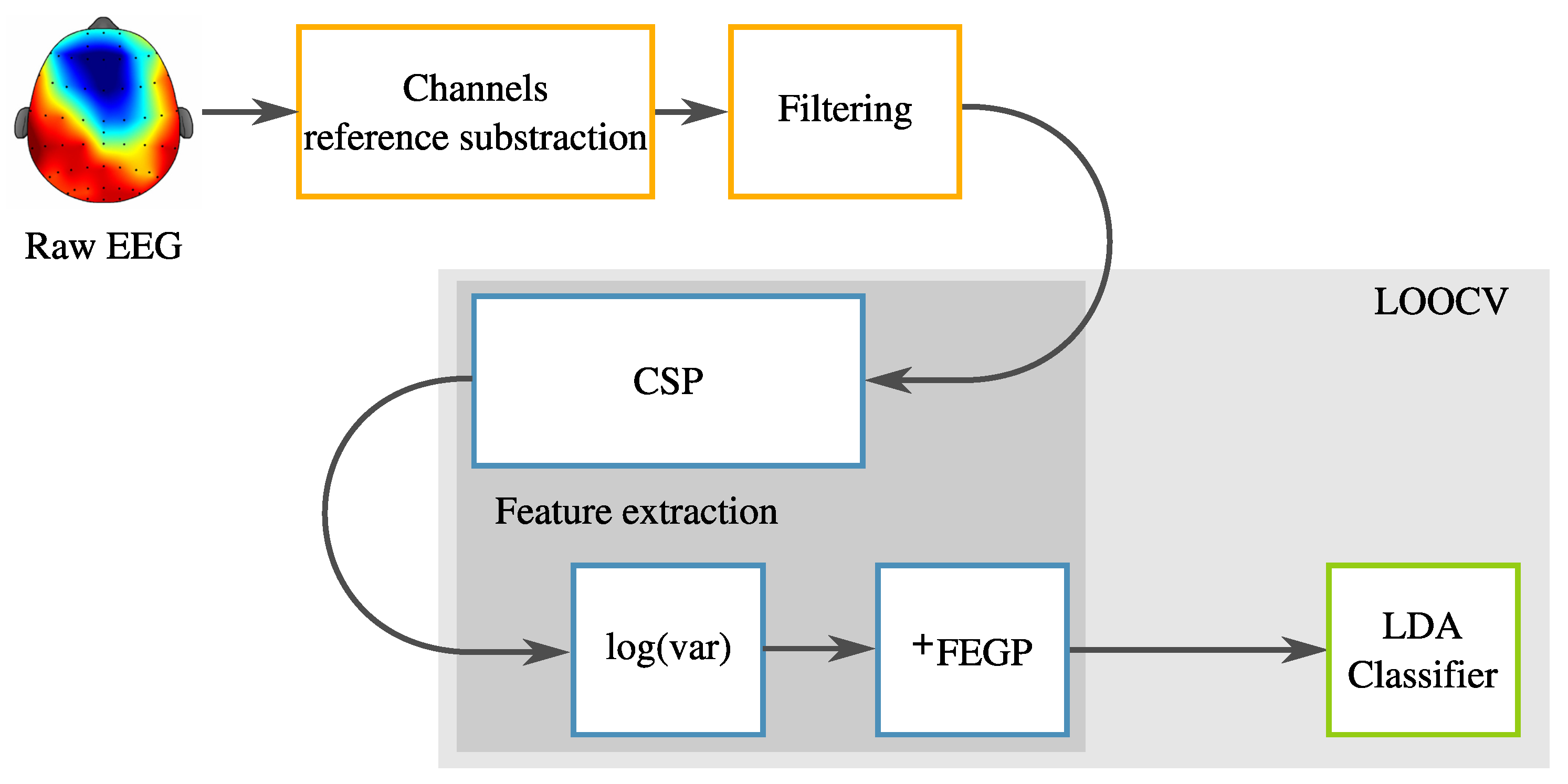
The reference system is essentially the first part of our previous work [9]. Particularly, a complete classification system is built based on several stages. First, a data acquisition protocol was followed. Second, a preprocessing step involving spectral filtering is applied. Third, a feature extractor based on the CSP is used. Finally, fourth, the classification task is solved with LDA. This reference system is summarized in Figure 1. In the following subsections, each of these elements is explained in detail.
2.1. Data Acquisition
2.1.1. Acquisition Protocol
A group of individuals (critical personal information was protected) participated in the experiments during a 2011 campaign at the Université de Bordeaux, France. Each person was subjected to the same procedure, which is summarized in the following paragraph, with more details given in [9].
The participants were put inside a soundproof room where the experiments were performed. A recording cap with 58 electrodes was placed over the scalp of each person. Then, a special session was executed, commonly referred to as Contingent Negative Variation (CNV) protocol [46], where the goal is to determine if the subject is truly in the appropriate physiological state. Two CNV tests were used, each one corresponding to a specific mental state. After each CNV test, the data used in this study were recorded for each subject. This procedure is further explained in [9].
2.1.2. Subjects
The experiment involved 44 subjects (mixed gender), non-smoking, aged from 18 to 35 years old. All are right-handed to avoid variations in the characteristics of the EEG due to handedness linked to functional inter-hemispheric asymmetry. After the CNV test, several subjects were rejected, since the CNV test determined that they did not reach the expected mental state. Therefore, only 13 valid individuals were used to build the dataset used in this work.
2.1.3. Raw Data
The recorded data, considered as the raw data in this study, contain 26 records of approximately three minutes each (13 corresponding to the normal state and 13 more for the relaxed state) of 58 channels for each subject. A sampling frequency of 256 Hz was employed during the acquisition with the Deltamed system. Since the length of the recordings slightly varies from subject to subject, approximately 46,000 samples were obtained for each recording.
2.2. Pre-Processing
For this type of system, the automatic detection should be accomplished by just analyzing a small portion of a signal and classifying it as quickly as possible, particularly in an online scenario. By splitting the signal into small packets of data (commonly referred to as trials), training, and testing, a supervised learning system is possible.
However, the length of a trial cannot be defined a prioril thus, a quick analysis to determine an appropriate size for the trials is required. In [9], different trial lengths were evaluated and the optimal one was found based on the classification accuracy. Lengths of 1024, 2048, and 4096 samples were analyzed, and a value of 2048 samples (eight seconds) was found to be the best, resulting in 22 trials per subject/class. Consequently, this value was also used in this work. Therefore, our dataset is stored in a matrix .
Recorded EEG signals usually contain noise and mixed frequencies. These mixed frequencies are partly due the oscillatory rhythms present in normal brain activity [47]. The most studied rhythms are alpha (8–12 Hz), beta (19–26 Hz), gamma (1–3.5 Hz), and theta (4–8 Hz), which are associated with different psycho-physiological states. The alpha waves are characteristic of a diffuse awake state for healthy persons, and can be used to discern between the normal and relaxed states. Actually, in some recordings, alpha waves begin to appear when the subject is starting to relax.
In this work, band-pass filtering is applied to discriminate frequencies outside the alpha and beta bands. Again, an analysis is required to find out which cutoff frequencies are useful to build the filter by sweeping a range of candidate values. In [9], we presented such an analysis, with the resulting values of 7 and 30 Hz corresponding to the low and high cutoff frequencies using a fifth-order Butterworth filter, matching what other researchers have found as well [48,49]. The filter response is illustrated in Figure 2.
2.3. Common Spatial Patterns
Like other techniques that derive a projection or transformation matrix based on some specific requirements (e.g., Independent Component Analysis (ICA) or PCA), the CSP is a technique where a matrix is built that simultaneously maximizes the variance of a multivariate subset with an arbitrary label and minimizes the variance for another subset with a different label. Projected data are given by , where is the data transformed from the original dataset into with dimensions , where p is the number of channels, n is the number of trials, and T the trials’ length for all subjects and two classes. is a filter matrix, as described below. This technique is useful in a binary classification problem because data are projected onto a space where both classes are optimally separated in terms of their variance.
The CSP can be briefly defined as the following optimization problem:
and
where is the matrix that contains the trials for class one and the matrix for class two, or, respectively, the normal and relaxed conditions in our case. Coefficients found in and define a set of filters that project the covariances of each class orthogonally.
This problem can be solved by a single eigen-decomposition of , where
is the estimation of the covariance corresponding to the average of trials of class one. Similarly,
is homologous for class two. In a single eigen-decomposition, the first k eigenvectors (corresponding to the k largest eigenvalues) of are also the last k eigenvectors of . Sorting the eigenvalues in descending order, we can build our filter matrix with
in which filters are considered pairwise () for . The number of filter pairs can greatly affect the classification accuracy; thus, a tuning step is needed to find the optimal number of filters. This step was performed in [9], resulting in a value of , which is employed in this work as well.
2.4. Classification
To approximate a normal distribution of the data, the logarithm of the variance obtained from the input data transformation by is calculated. This is stored in a matrix , and is given by
where is a vector from the matrix spanning the 58 electrodes, , is a vector from the matrix with length 58, and . The evaluation of the classification process is performed using the Leave-One-Out Cross-Validation (LOOCV) method. In this methodology, data are split into q folds (), where the training subset has a size of and the testing has a size of one. In our case, , the number of subjects. The process is repeated q times by changing the index m for testing and keeping the remaining folds for training. The reason for using this type of partitioning is because the recognition is performed at the individual level (grouping trials from the same individual) rather than at the trial level. We want to avoid training and testing the classifier using trials from the same subject, which could lead to misleading results.
The classifier used is LDA. This technique is commonly used in BCI systems due to its ease of implementation and competitive performance compared with more sophisticated algorithms [50]. Briefly, in LDA, a hyperplane is calculated based on the covariances of the data distribution, and it optimally separates two classes. If we assume that both classes belong to a normal distribution and have the same covariance, then we can calculate
and
where is the shared covariance matrix for both classes, while and are the corresponding means for each class. Classification is performed by assigning a label (either C1 or C2) to a label vector depending on a score vector , given by
and
Until this point, we employed the training data to obtain the CSP filter set and the vector . During the testing phase, a prediction vector is computed using the hyperplane found during training but using a projected testing data based on the pre-calculated .
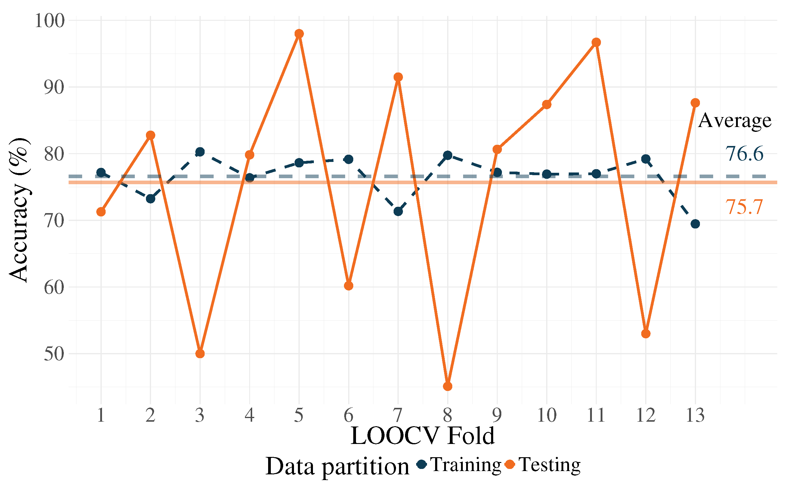
Since this is calculated for a given fold in the LOOCV procedure, after q repetitions, an average of the accuracy results of all folds is computed and is considered as the prediction accuracy. Results from the classification performance can be seen in Figure 3, where the average and fold-wise accuracy are presented corresponding to the training and testing partitions. For training, an average accuracy of 76.6% was obtained, and 75.7% for testing. Please note that over-fitting exists (or a failure to generalize) for some folds, namely 3, 6, 8, and 12.
3. Proposed Enhanced System
In this section, we present a novel algorithm based on GP that extends the reference system to improve the classification results, particularly for the prediction over unseen data. From a general point of view, the enhanced system is described in Figure 4, where it can be seen that the proposed Feature Extraction with GP (FEGP) follows the CSP block. In other words, we perform a post-transformation of the CSP output, with the goal of improving the classification results.
3.1. Genetic Programming
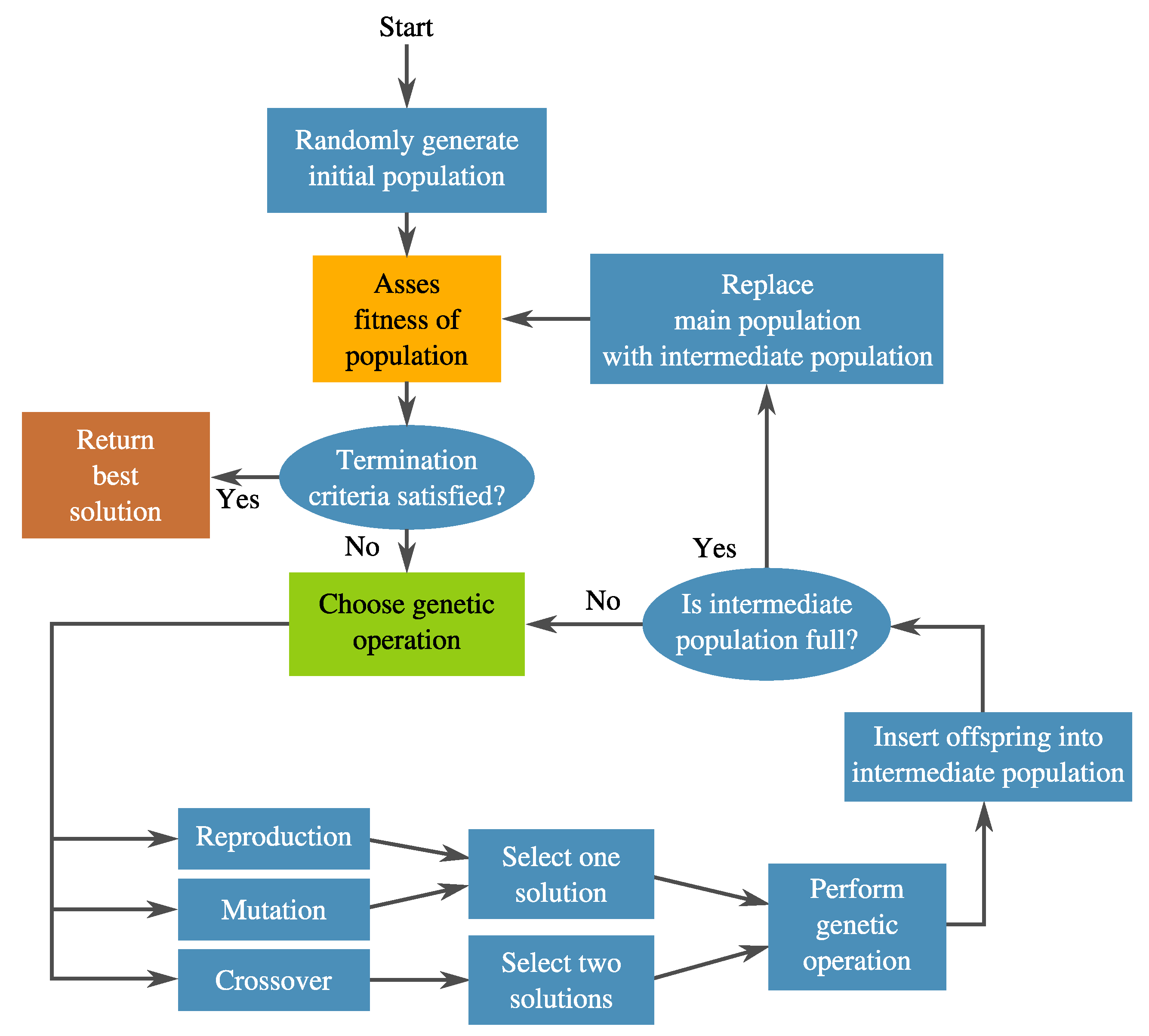
As a segment of the broader Evolutionary Algorithms (EA) research area, GP [51] is sometimes considered to be a generalization of the popular GAs [52]. In GP, a pool of candidate solutions (population) are syntactically evolved towards a specific objective by applying selection pressure based on a quality assessment or fitness, which are normally driven by an objective function. GP differs from other population-based algorithms on the following fronts. First, the solutions or individuals are expressed with a symbolic structure. This is mainly where its strength comes from, since it can represent many things depending on the problem’s domain. The only restriction is that the expression must be computable, which is to say, for a given input, it produces a valid output. Second, the size of the solution is variable, meaning that during the search, the length or size of solution candidates changes. This provides GP its second strength—solution structures are not predefined; rather, they are evolved simultaneously with their performance. A general diagram for GP is presented in Figure 5.
GP has been used successfully in many applications with different representations [53], but the tree representation is the most common among them—the same representation used in this work.
Although the canonical GP has achieved competitive performance compared with other algorithms [40,53], including hand-made designs, it is not suitable for all types of problems, especially when the underlying data have complex properties. GP performance depends on the underlying data complexity, which, for some problems, could lead to a search stagnation or premature convergence [54]. Another shortcoming for GP, also present in other machine learning algorithms, is model over-fitting in under-sampled data [55]. There are several ways to improve the over-fitting issue, like using a validation partition with an early stopping of the training process, or using a regularized objective function [56]. To use a validation partition means that data size has to be sufficiently large, which is not the case in the currently studied problem, so the most reasonable approach was to use a regularization approach. For these reasons, a new algorithm is proposed based on an extension of previous works [10,57].
3.2. Augmented Feature Extraction with Genetic Programming: FEGP
Recognized as one of the most important tasks in a classification system, our main proposal is focused on the improvement of the feature extraction stage. One of the discovered complexities found during the implementation of the reference system is that the data of the study are highly varied and uncorrelated within the same class, and overlapped between both classes. This yields a non-trivial problem for any supervised learning system. A suitable strategy would be to build a non-linear model that produces new features, which further increase the inter-class distance and reduce the intra-class dispersion.
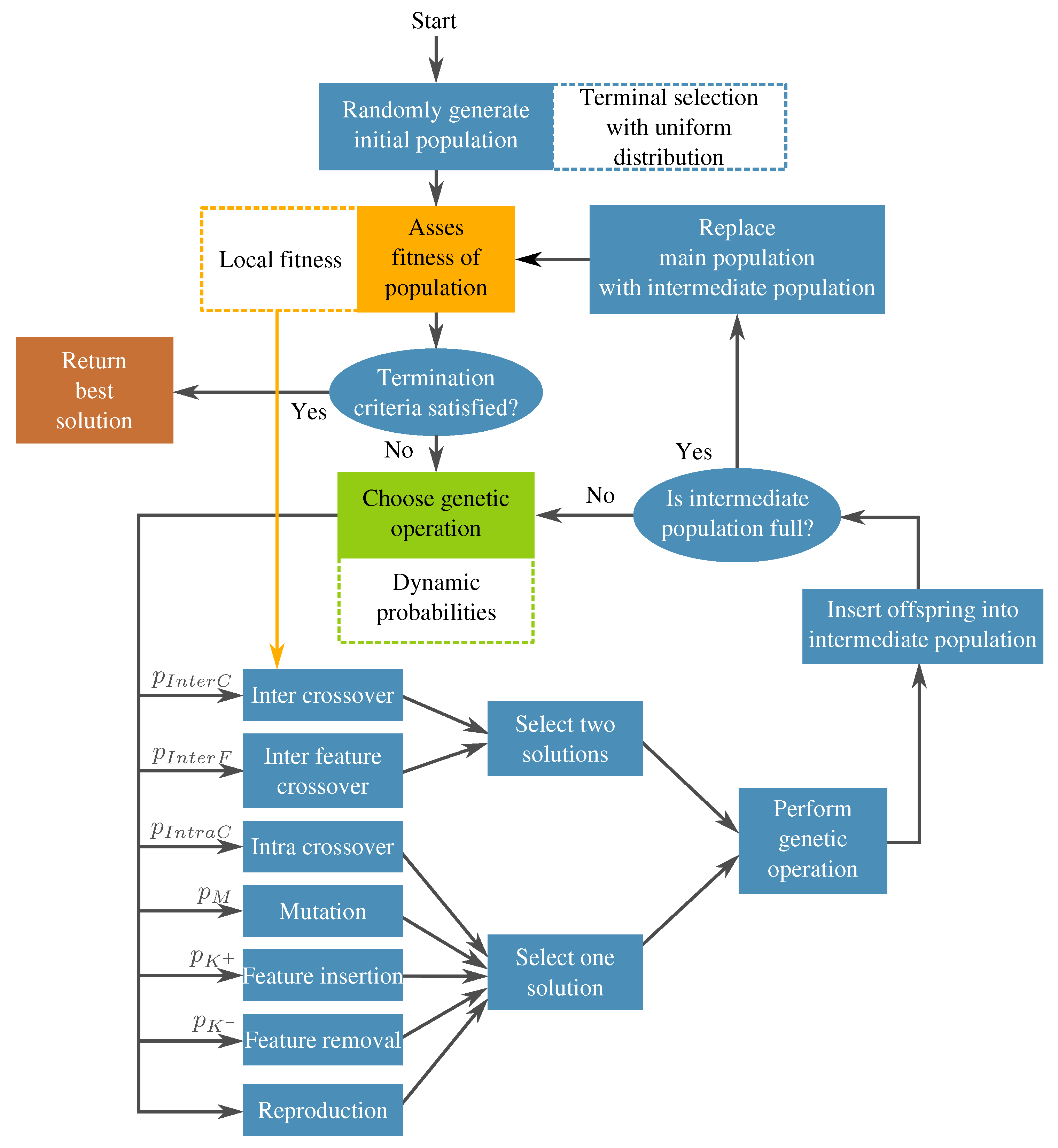
Based on this, a GP-based algorithm is proposed with the objective of improving the classification accuracy for the reference system. Another goal for the proposal is to be highly flexible, not explicitly depending on any specific pre-processing or classifier blocks. A diagram for this algorithm is depicted in Figure 6, hereafter referred to as FEGP, for augmented Feature Extraction with GP.
Similar research on feature extraction with GP has been conducted. Guo et al. [25] proposed first an individual representation with a single root node, where a special node called ’F’ can be inserted into any part of the tree, which produces a new feature. Other than this enhancement, no special search operators were used for their system. On the other hand, Firpi et al. [58] used a canonical GP individual representation, where a single tree produces a new feature, a rather simple proposal that nevertheless produced competitive results for the classification of signals from epileptic seizures. A similar approach was followed by Poli et al. in [59], where a single root node representation with a custom fitness function was used to evolve mouse trajectories by employing EEG signals. The authors used a strongly typed GP, a variant in which there is an explicit constraint on the data type allowed in the terminals and functions. In a previous work [40], we used GP as a classifier for the detection of epileptic stages, taking as input simple statistics from each trial.
The present proposal builds upon previous works in [10,57], where the Multidimensional Multiclass Genetic Programming (M3GP) algorithm was presented. M3GP also uses some additional search operators to add or remove complete features during the run, but mostly relies on a canonical GP implementation with a single objective function that only takes into account the training accuracy and a static parametrization of the GP settings. On the other hand, FEGP includes a wider variety of search operators, a specialized local fitness measure to account for the fact that each solution is a collection of subtrees, dynamic parameters that control how the search is performed at different moments during the evolution, a regularized fitness function to control over-fitting and achieve better generalization, and a specialized initialization procedure to account for the extremely large feature space in this problem domain. Each of these features will now be explained in greater detail.
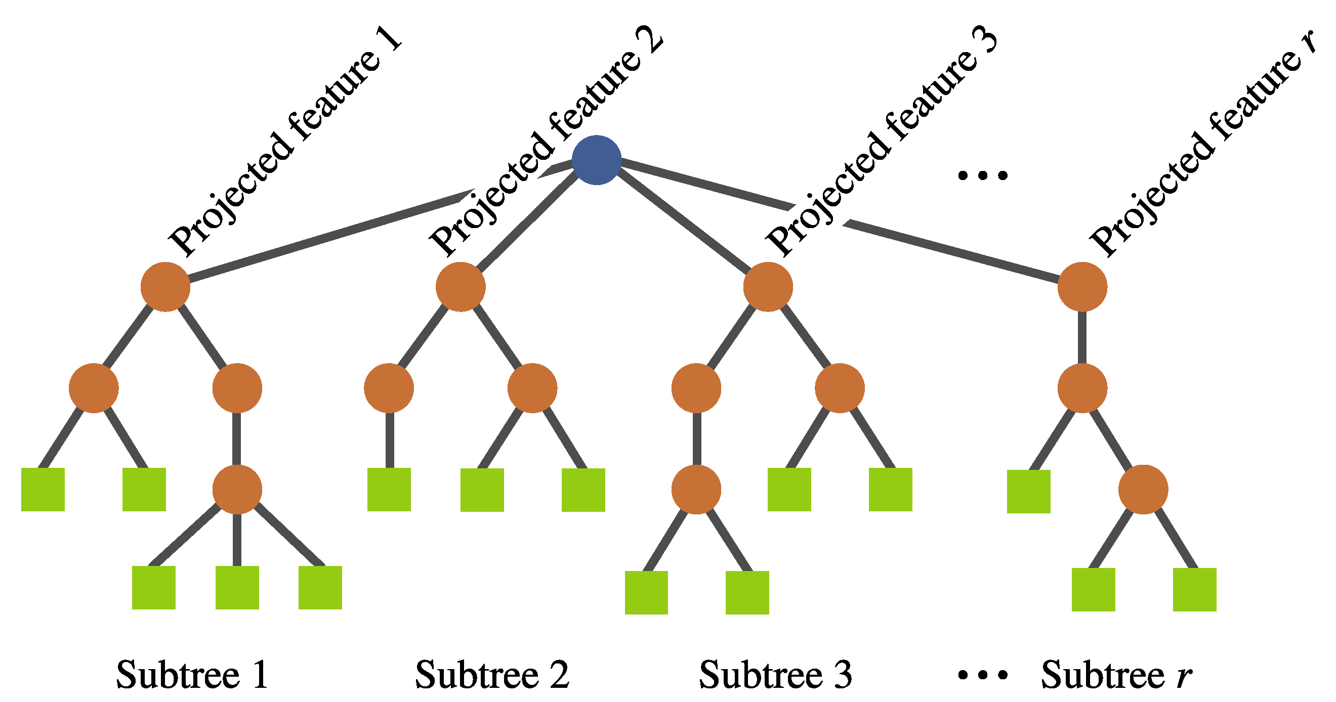
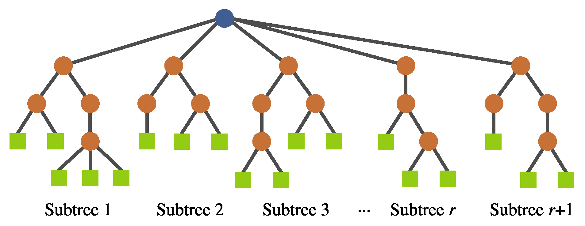
- Individual representation. The representation is also based on a tree structure, but it involves a multi-tree with a single root node, such that each individual defines a mapping of the form , where k is the number of input features and r is the number of newly constructed features. Each of these subtrees are constructed in the same way as in a canonical GP (see Figure 7). No calculation is executed at the root node; it is rather used as a container for the output of the evolving r subtrees. Each subtree works as a non-linear transformation of the input features into a new space that is expected to simplify the classification. Moreover, the number of new features r can vary among individuals.
- New genetic operators. Because of the manner in which individuals are represented, it is necessary to introduce new search operators. For any of these operators, the root node is avoided during the operation to preserve the representation.
- (a)
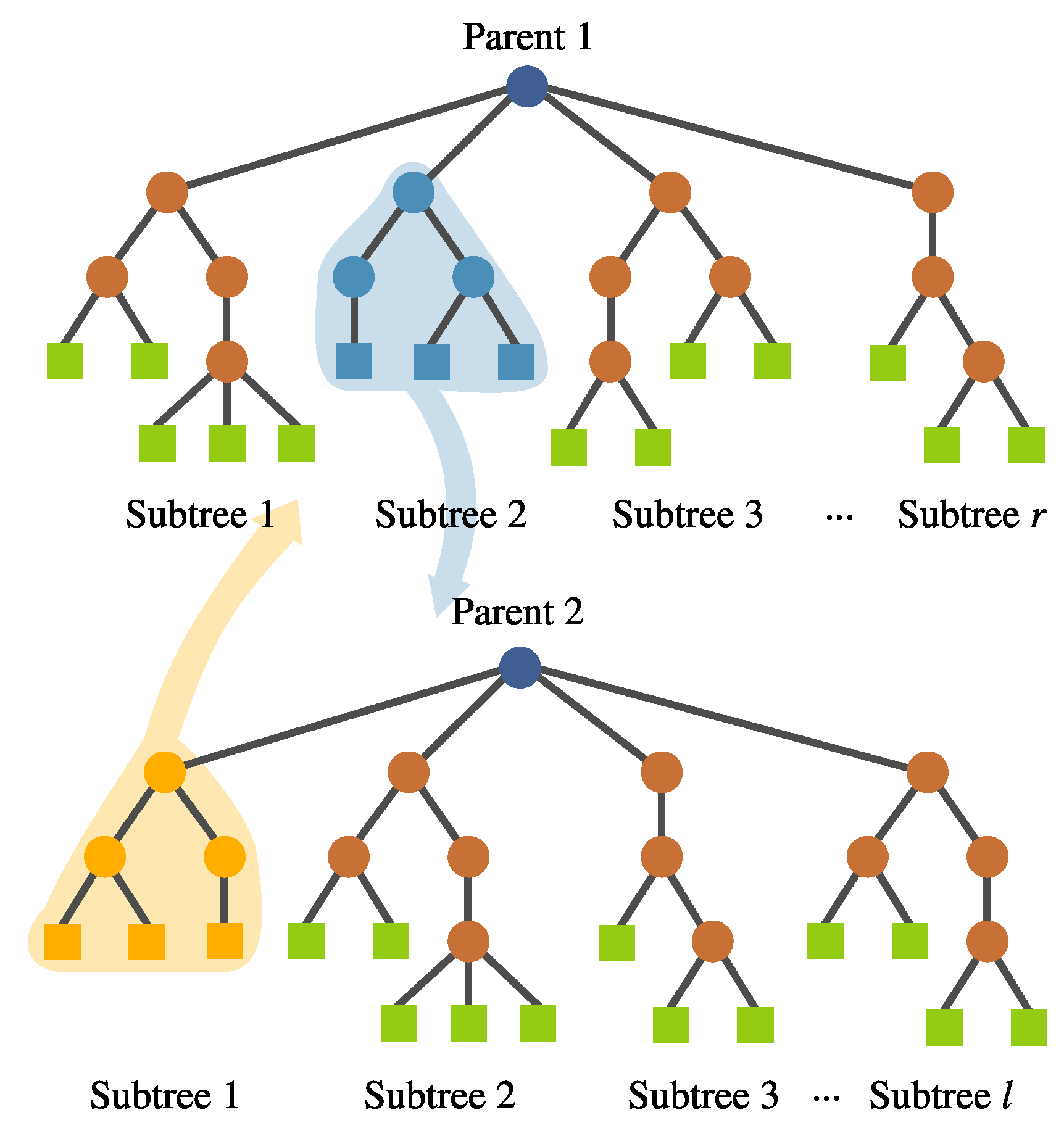
- Inter-crossover. This is a crossover performed between subtrees belonging to different individuals, which produces two offspring. The selection for the crossover points is based on a local fitness measure (discussed in detail later), which allows the best subtrees to interchange genetic material. This is visualized in Figure 8.
- (b)
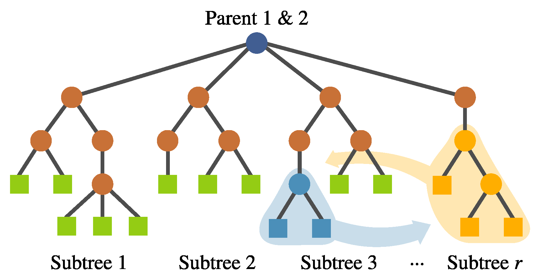
- Intra-crossover. For a given individual, genetic material can be swapped within the same individual using this operator, depicted in Figure 9. The rationale behind this is that genetic material from one feature might help the evolution of another within the same individual, improving the overall fitness. The subtree selection is performed randomly, choosing the crossover points from different subtrees. This operator generates two offspring.
- (c)
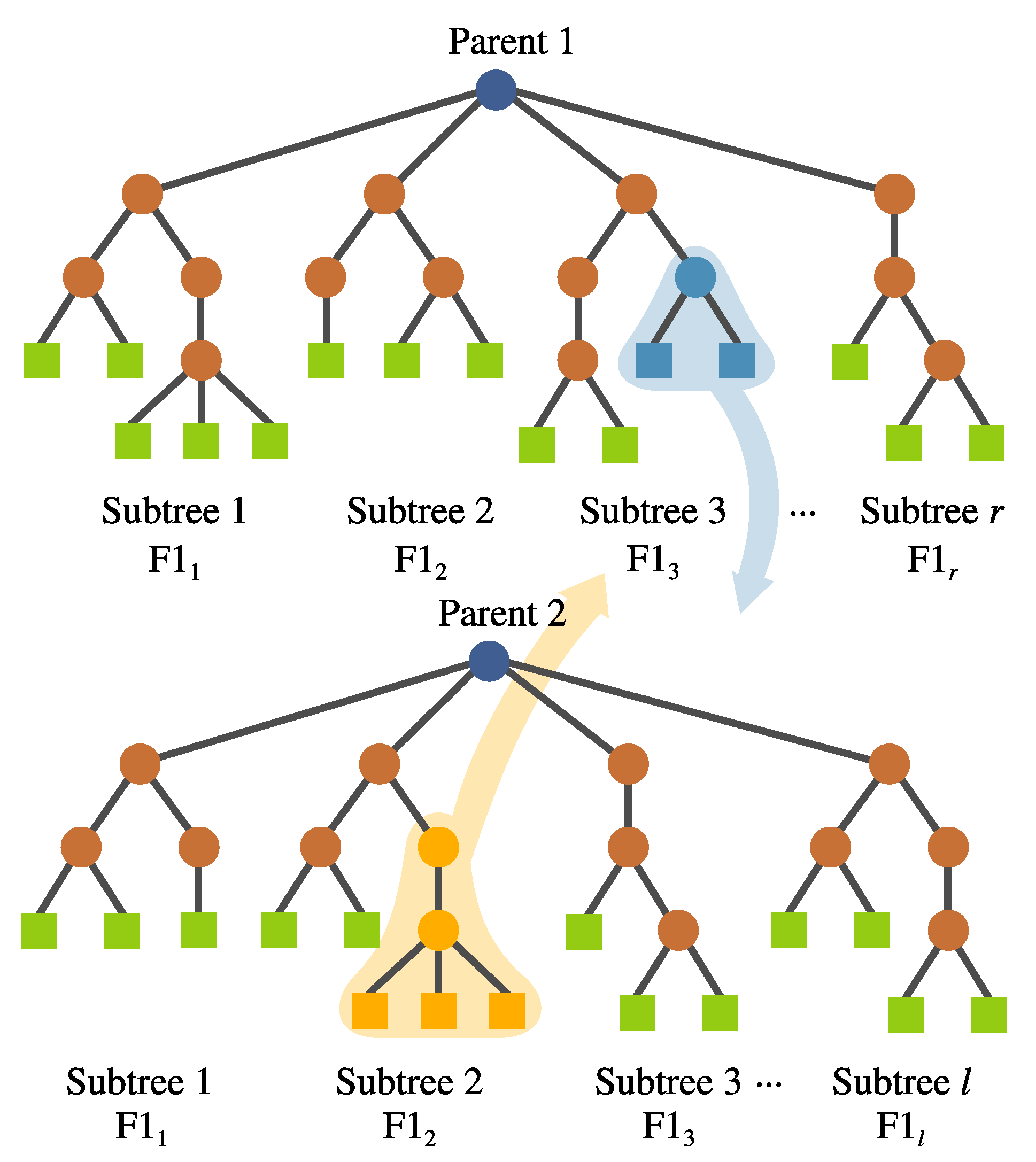
- Inter-individual feature crossover. It can be desirable to keep complete features with good performance within the population. This operator interchanges complete subtrees between two selected individuals. This is performed randomly rather than using a deterministic approach. Preliminary experimentation suggested that avoiding a fitness-based selection of the subtree allowed the algorithm to explore the solution space better. This operator can be seen in Figure 10.
- (d)
- Subtree mutation. This is performed the same way as in canonical GP. A portion of a selected subtree is substituted with a randomly generated tree.
- (e)
- Feature insertion mutation. This operator allows the insertion of a new randomly generated subtree, expanding the dimensionality of the transformed feature space; Figure 11 depicts this operator.
- (f)
- Feature removal mutation. Similarly, a deletion operator is needed to reduce the new feature space. The subtree to be removed is selected randomly. This operator can only be used if .
- Terminal selection during population initialization. In a canonical GP, the initial trees are built by randomly choosing a function or terminal from the available sets in an iterative fashion. This selection process is commonly referred to as sampling with replacement, which could lead to some variables not being chosen as terminal elements in the initial population; the probability of this happening will increase when the number of input features is large. If this is the case, then the initial generations will lack proper exploration of the search space, particularly in the terminal elements, which may lead the search toward local optima. A simple mechanism to avoid this is to enforce that every variable is chosen at least one time as a terminal element in a GP individual. This can be achieved by performing a sampling without replacement of the input features in the terminal set of the GP search. When a terminal is randomly selected, then it is excluded on the subsequent terminal selection steps until all available terminals have been chosen; then, the procedure is repeated by making all terminals available to the tree generation algorithm, such as full, grow, or Ramped Half and Half.
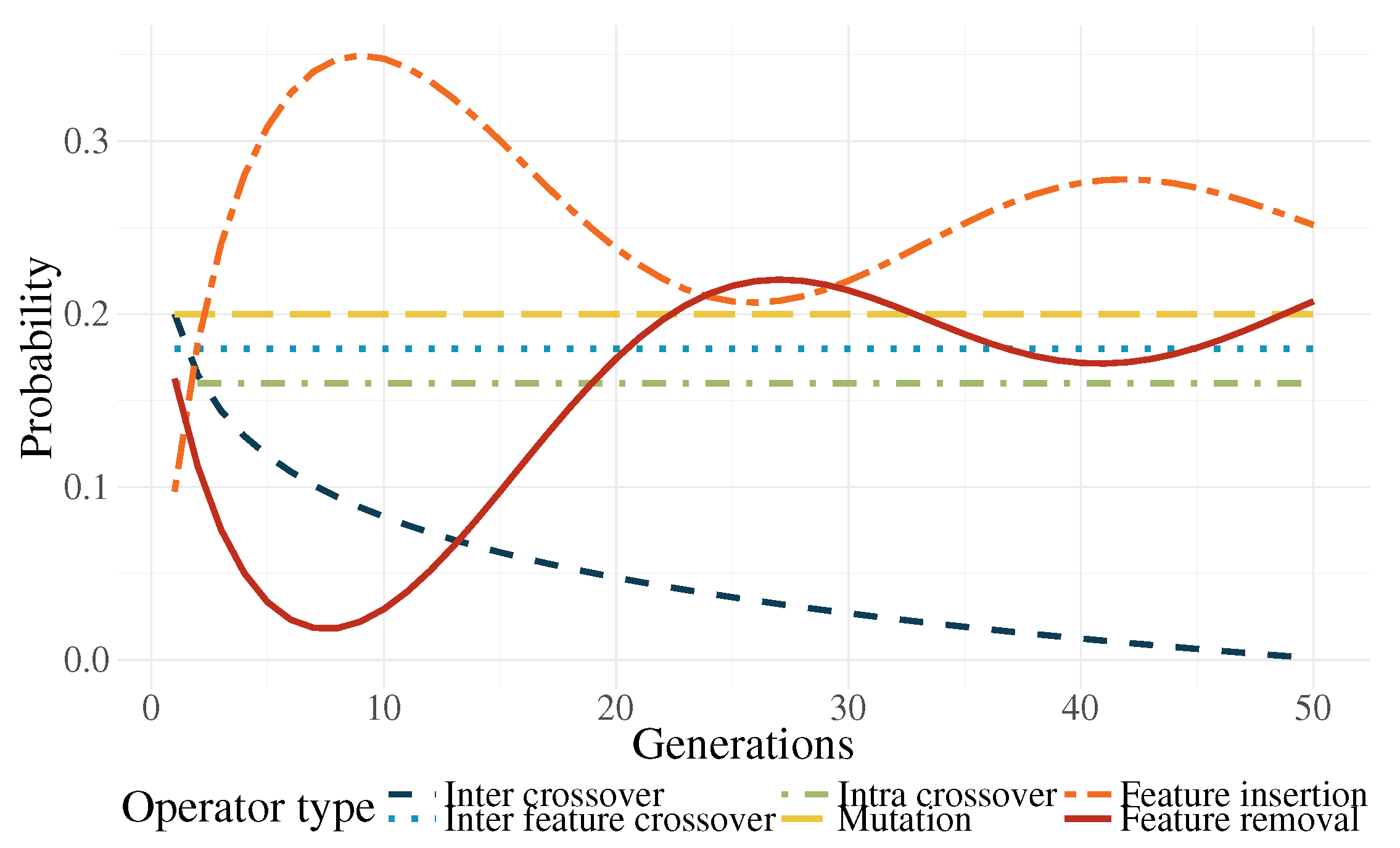
- Genetic operator selection. In canonical GP, operators are chosen at each generation with a user-defined probability. The probability of choosing each operator is usually static throughout the search. In the work by Tuson and Ross [60], their operator probabilities are changed at each generation by rewarding or penalizing operators according with their success at producing good offspring (offspring with high fitness). After an initial preliminary experimentation, we propose functions that modify the operator probabilities based on the work of Tuson and Ross.Based on [60], three operator probabilities (intra-crossover: , inter-individual feature crossover: , and subtree mutation: ) are given by a common dynamic behavior, with the following characteristics: They are periodic, the variation range is rather small, and they are stationary. For simplicity, this condition was replaced by a constant value; in early experimentation, the system behaved almost identically to the algorithm by [60].The other three operators (inter-crossover: , feature insertion mutation: , and feature removal mutation: ) exhibited unique dynamic behaviors using the algorithm by [60]. Here, we proposed the following equations to mimic the behavior of the aforementioned algorithm:where is the current generation, is the maximum generation number, is a decay parameter, and is an initial probability. In preliminary tests, it was found out that, only in the earlier generations, a high probability for the inter-crossover operator was required, mainly to promote the exchange of genetic material and allow the algorithm to do a more efficient search. In more advanced stages of the evolutionary process, this operator produced a negative effect in the search by curtailing the ability of the algorithm to perform exploration. As a countermeasure to this phenomenon, the selection probability for this operator is reduced.Two of the most important operators are the feature insertion and removal mutations. Indeed, these are the ones responsible for the flexibility of the new feature space size. There is a higher probability that the hyperplane of the classifier has a good class separability when the number of dimensions is high. A high probability for the generation of new features () at the start of the run promotes the search for the most promising size of the new feature space. The ratio between these operators and the static ones decreases after the initial generations, giving more importance to the evolution of the solutions without changing the feature space too much. Because evolved models stagnate at the end of the run, increasing the feature space size is required once more. Moreover, (features removal) is seen as the complementary part of and . The operator functions are plotted in Figure 12 for the case that .
- Fitness calculation. The fitness is computed by a local and a global measure, which are used differently by the search. More specifically:
- (a)
- Local fitness measure (Fisher’s Discriminant Ratio). This is computed at the subtree level, which provides a separability value for each constructed feature. Certainly, the quality of a solution depends on the quality of their individual features. The local measure is only used as the criterion for the inter-crossover subtree selection, that is, crossover points are selected within the subtrees with the best local fitness. Although the GP selection process chooses two individuals with similar fitness rank, it does not guarantee that all individual subtrees have a good performance. The goal is for the crossover to exchange features that show good performance in terms of class separation. This is given bywhere , , , and are the means and standard deviations corresponding to class one and two for the ith feature [61]. For any given tree K, r local fitness measures are calculated. It was found that the use of the local fitness in other operators did not help the search.
- (b)
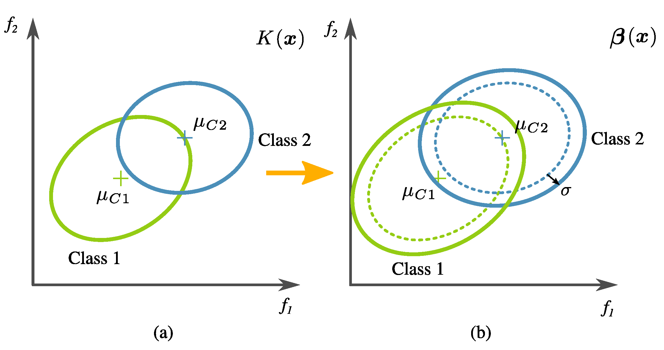
- Global fitness measure. The calculation of global fitness is the result of a two-tier process.In the first level, an initial regularization is performed over the tree output using the training data; then, the classification accuracy () is calculated. In detail, this is done by artificially changing the covariance of transformed training data (i.e., the training data in the new feature space created by an evolved transformation), defined byandwhere denotes the tree output corresponding to all the data samples from class (normal), and is the same but corresponding to class (relaxed). The main reason for this is that data variance is high in this problem, and the classifier training has to be relaxed so that prediction accuracy on unseen data increases. Please note that the actual penalty is given by a factor of twice the standard deviation of the transformed training data. This is exemplified in Figure 13. The confusion matrix is calculated using LDA over the modified data. The classification accuracy is specifically computed withwhere TP (True Positive), TN (True Negative), FN (False Negative), and FP (False Positive) are values from the confusion matrix as a result of the labels .In the second level of the two-tier process, the global fitness is computed bywhere is a proposed second regularization term, given bywhich becomes zero if FP and FN are equal. In preliminary experimentation, it was found that the algorithm tended to avoid over-fitting when there was a balance in the FN and FP scores.
Finally, it is important to mention that although the LDA classifier was used during training, it was meant only for driving the search so the class separability would increase. Once FEGP finds a new transformation model, any classifier can be used during testing. This offers flexibility in terms of the classifier choice, especially when dealing with a broader range of classification problems.
4. Experimentation and Results
In this section, we present experimental details regarding the proposed system. The reported algorithms were implemented in MATLAB. Specifically for the FEGP algorithm, the GPLAB (http://gplab.sourceforge.net/) [62] toolbox was used as a starting point for the implementation. The experiments were executed in a setup with an Intel Xeon at 2.4 GHz with 32 GB of RAM.
Given the stochastic nature of GP, a series of multiple runs were executed in order to statistically determine the algorithm performance. Following the LOOCV scheme for data partitioning and validation, the experiments involved 30 independent runs for each fold. The results presented in this work contain 390 runs in total (). Details of the values used for filtering, CSP, and LDA were mainly discussed in Section 2. Furthermore, the FEGP parameters are summarized in Table 1. Some comments in the third column are derived from experimental tuning of the algorithm.
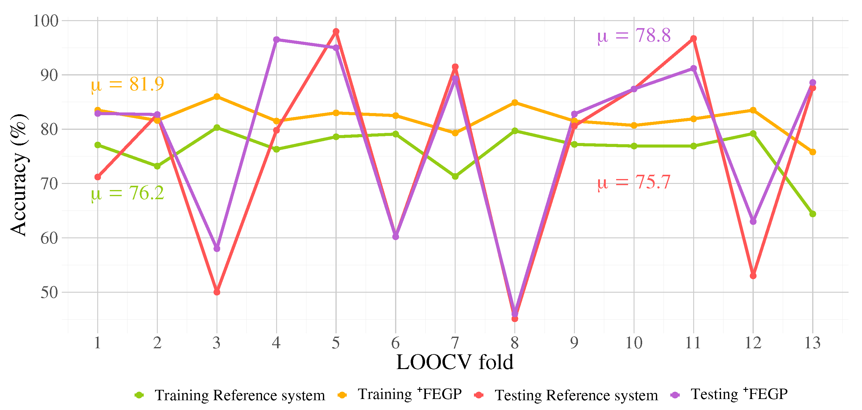
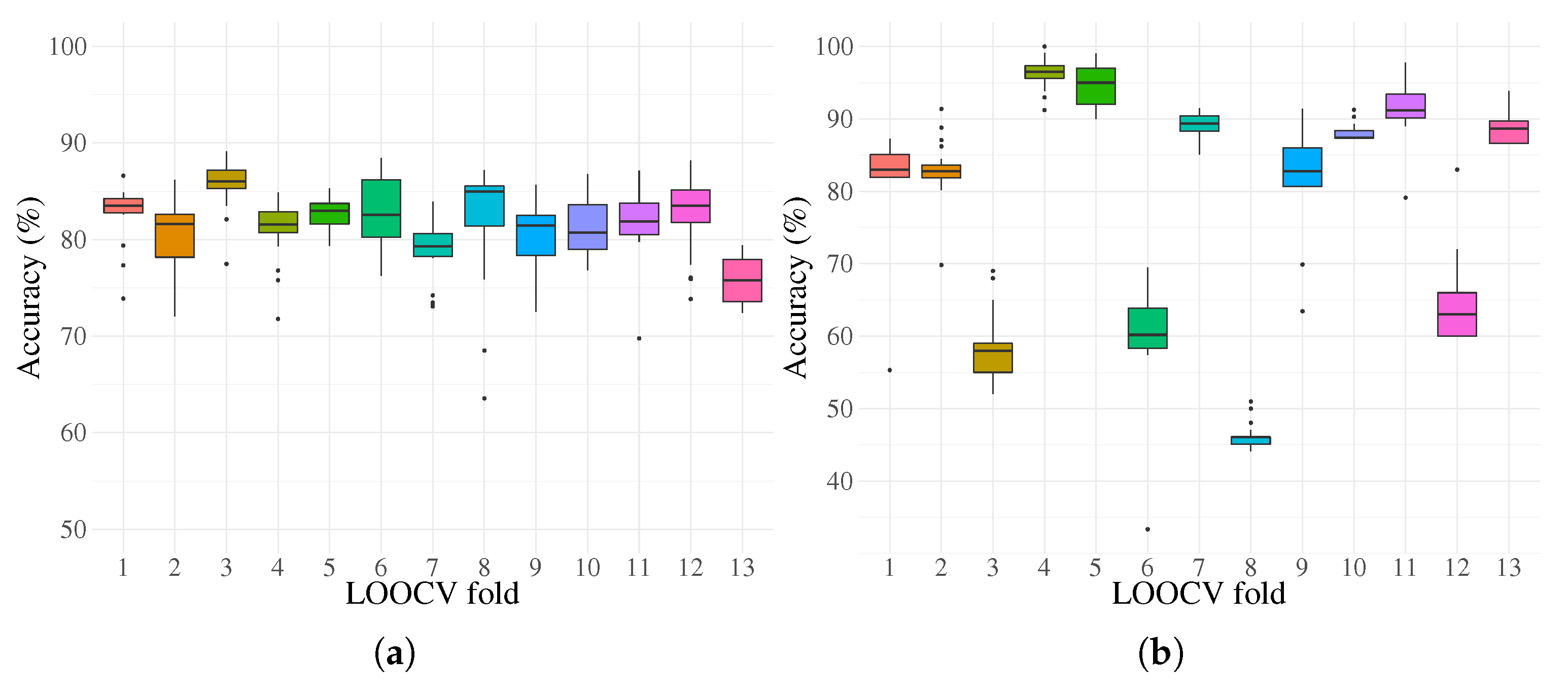
The training classification performance of the proposed enhanced system is shown in Figure 14 with the overlapped performance of the reference system for comparison. In addition, the predictive performance calculated over the testing partitions is presented in Figure 14. Basic statistical results for the FEGP-based system per LOOCV fold are given in Figure 15. Supporting these visual representations, the average classification accuracies and Cohen’s kappa values are presented in Table 2. To validate our results, non-parametric two-sample Kolmogorov–Smirnov and Wilcoxon rank sum tests were used to calculate pairwise statistical differences at a LOOCV fold level. The results are presented in Table 3 and Table 4, corresponding to the training and testing phases.
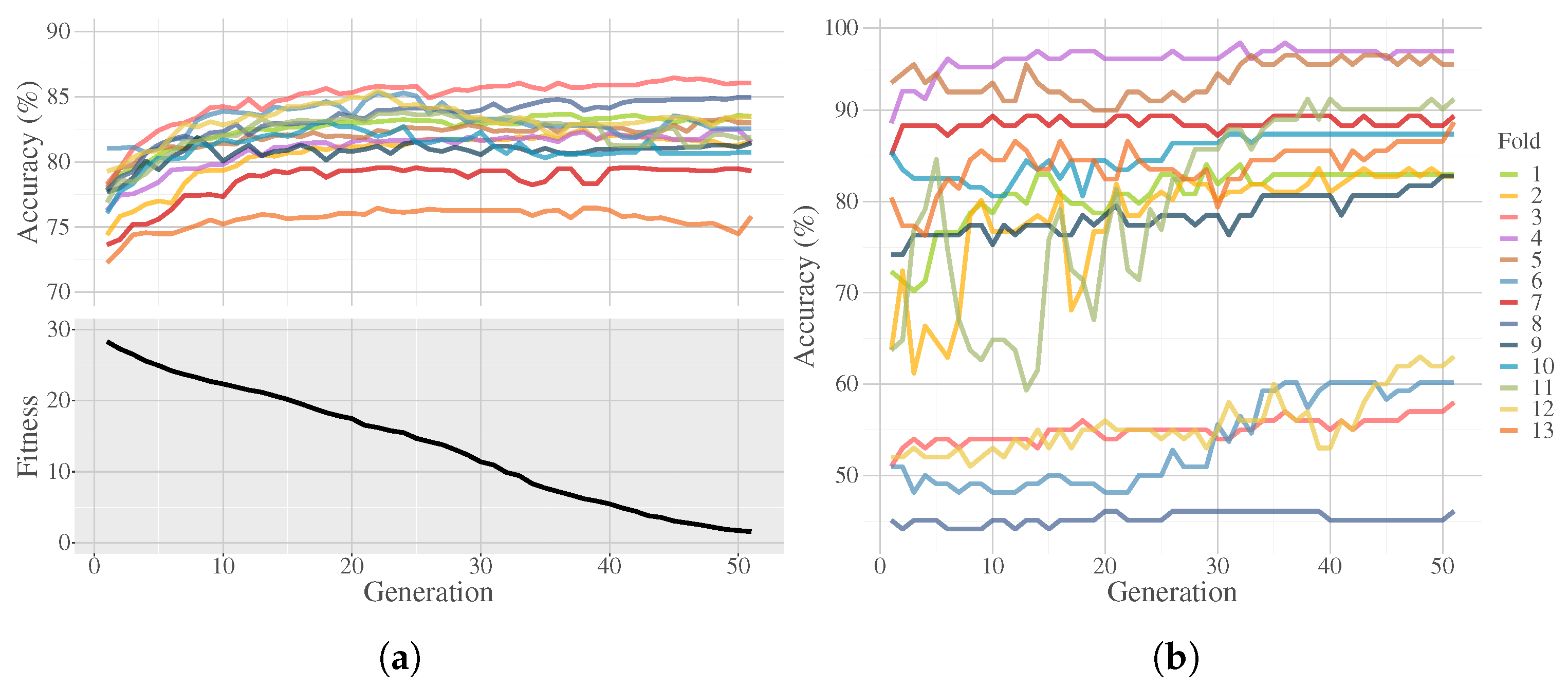
FEGP fitness performance and LDA classification accuracy during the training phase are shown in Figure 16a. Although the FEGP algorithm only uses the fitness measure (bottom plot), the top plot shows the convergence of the actual classification accuracy achieved by LDA across the generations. Please note that the bottom convergence plot condenses all 390 runs by first computing the median of 30 runs per fold and finally calculating the mean of all fold results. Similarly, in Figure 16b, prediction performance in terms of classification accuracy is presented as well.
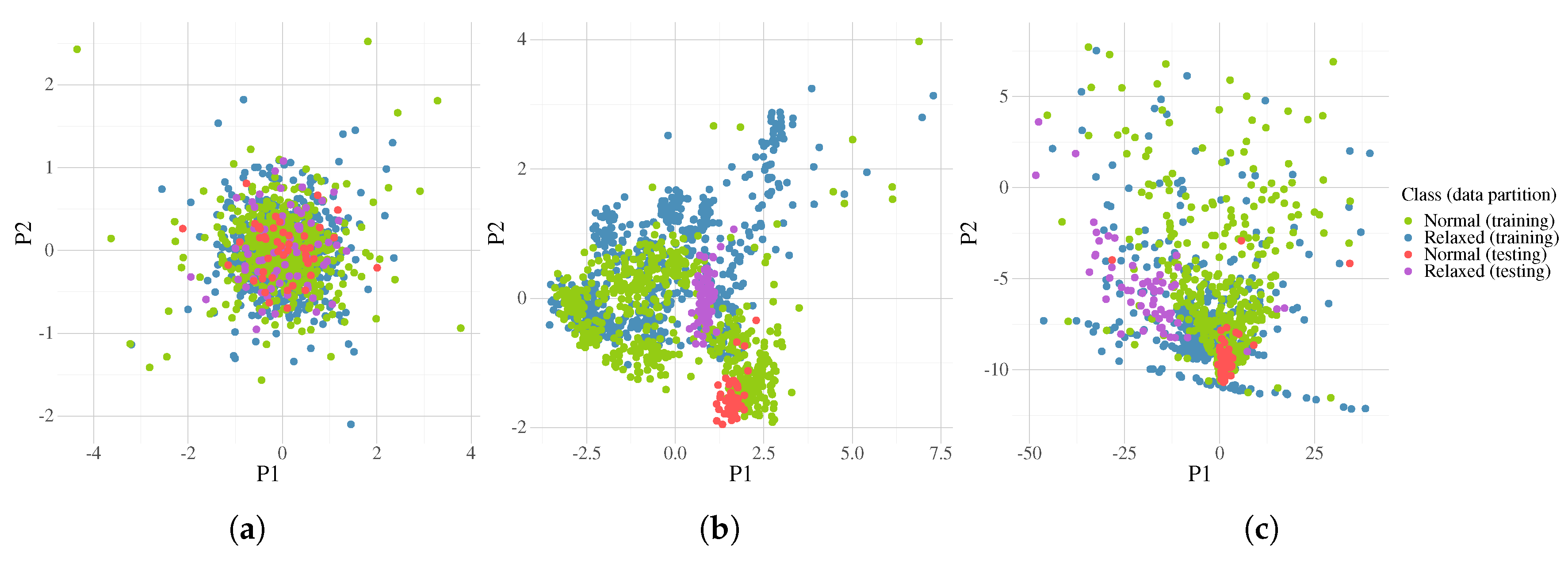
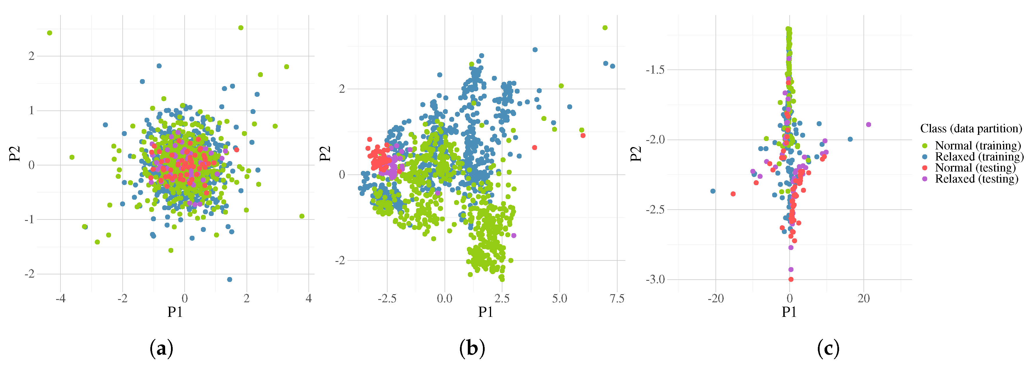
In order to provide a simple visualization of the data organization, a Principal Component Analysis (PCA) was calculated at different stages of the methodology. Two examples of the data distribution of each class are depicted in Figure 17 and Figure 18, corresponding to the folds with the best and worst performance on the testing data. The left scatter plots show the first two principal components from PCA calculated over the raw signals. The middle plots correspond to the data after the CSP (matrix ) calculation. Note a slightly different distribution between both folds because the CSP is performed with different training data. The plots on the right depict the data distribution after a randomly chosen run of the FEGP algorithm. The classification accuracy for Figure 17 is 82.8% for training and 99.1% for testing. The homologous values for Figure 18 are 81.4% (training) and 44.1% (testing).
5. Discussion
One of the main contributions of this work is the proposed feature extraction method, FEGP. Generally speaking, the classification accuracy in the training phase, as seen in Figure 14, surpasses the reference system. Furthermore, the system’s classification accuracy on unseen data also improved upon the reference system, as seen by the testing performance reported in Figure 14.
If we take a look at the system performance for each fold (Figure 15), we immediately see that some data partitions lead to better classification accuracies than others. Figure 17 and Figure 18 show the best and worst cases in terms of quality in more detail. After dimensionality reduction with PCA, we can recognize that the area of the overlap region for both classes is high in both cases for the raw data. Intuitively, we can deduce that for the majority of state-of-the-art classifiers, the performance will be poor in such circumstances. The effectiveness of CSP can be clearly seen afterwards, with a substantial increase in the separability of the classes. At this point, we can see that the testing cluster is quite different between almost all folds, with fold 4 and 8 being the extreme cases. For fold 4 (Figure 17), the testing data match the distribution of the training data, making it easier for a classifier to obtain good generalization results. On the other hand, in fold 8 (Figure 18), the case is the opposite; the data cluster belongs to a multi-modal distribution, where the obtained model is evolved over a different mode from that where the testing data reside, suggesting that the EEG recordings for that particular subject are quite different from the rest. Let us recall that although the experiments were done in a controlled environment, we could fully constrain the physiological activity of each subject. This is a more realistic scenario, but it makes the problem more difficult to solve. Furthermore, we can see the benefits of the FEGP algorithm in the third scatter plot of each figure. For fold 4, the new features make the problem quite trivial for almost any classifier. The robustness here is that the testing data do not shift or vary; rather, they integrate into the counterpart training samples. The more difficult case is fold 8; given an already problematic situation from the CSP output, the FEGP improvement is relatively small. Here, an important observation is that even for this worst case, the FEGP performance is at least the same or better, but not worse than the performance of the reference system.
We can further analyze the performance for the remaining folds in the LOOCV. The Wilcoxon test infers that the majority of the folds have a similar statistical performance in terms of their medians in the training phase, with the exception of folds 3 and 13. Although these are the extreme cases for training, their performance is an improvement upon the CSP output. This can be extended to all folds; indeed, FEGP produced an almost consistent improvement over all folds compared with the reference system. In the testing phase, almost all null hypothesis combinations were rejected, something expected given the nature of CSP output. However, the improvement was not linear among all folds. In folds 1, 3, 4, and 13, the improvement by FEGP was significant, but in folds 5, 7, and 11, there was a reduction in performance, suggesting that the obtained models were slightly over-fitted. Moreover, according to the Kolmogorov–Smirnov test, the hypothesis that samples from the algorithm’s outcome belong to the same distribution was not rejected for almost all folds during training, with the exception of folds 3 and 13 if we compare them with the rest. During testing, the hypothesis was rejected for almost all combinations. The statistical tests for the kappa scores support that the accuracy results are not influenced by a random phenomenon, with exceptions for folds 3, 8, and 12 on the testing performance, hinting that there is a small disagreement between the ground truth and the predicted labels.
The performance of the enhanced system can be seen from different angles. In the bottom plot of Figure 16a, we can see a steady minimization of the global fitness. At the same time, we can analyze the performance of the LDA classifier calculated directly over the transformed data. Although the training fitness is decreasing during the evolution, especially at the end, the classification accuracy does converge, and more importantly, the accuracy on unseen data does not decrease in the final iterations of the search (Figure 16b).
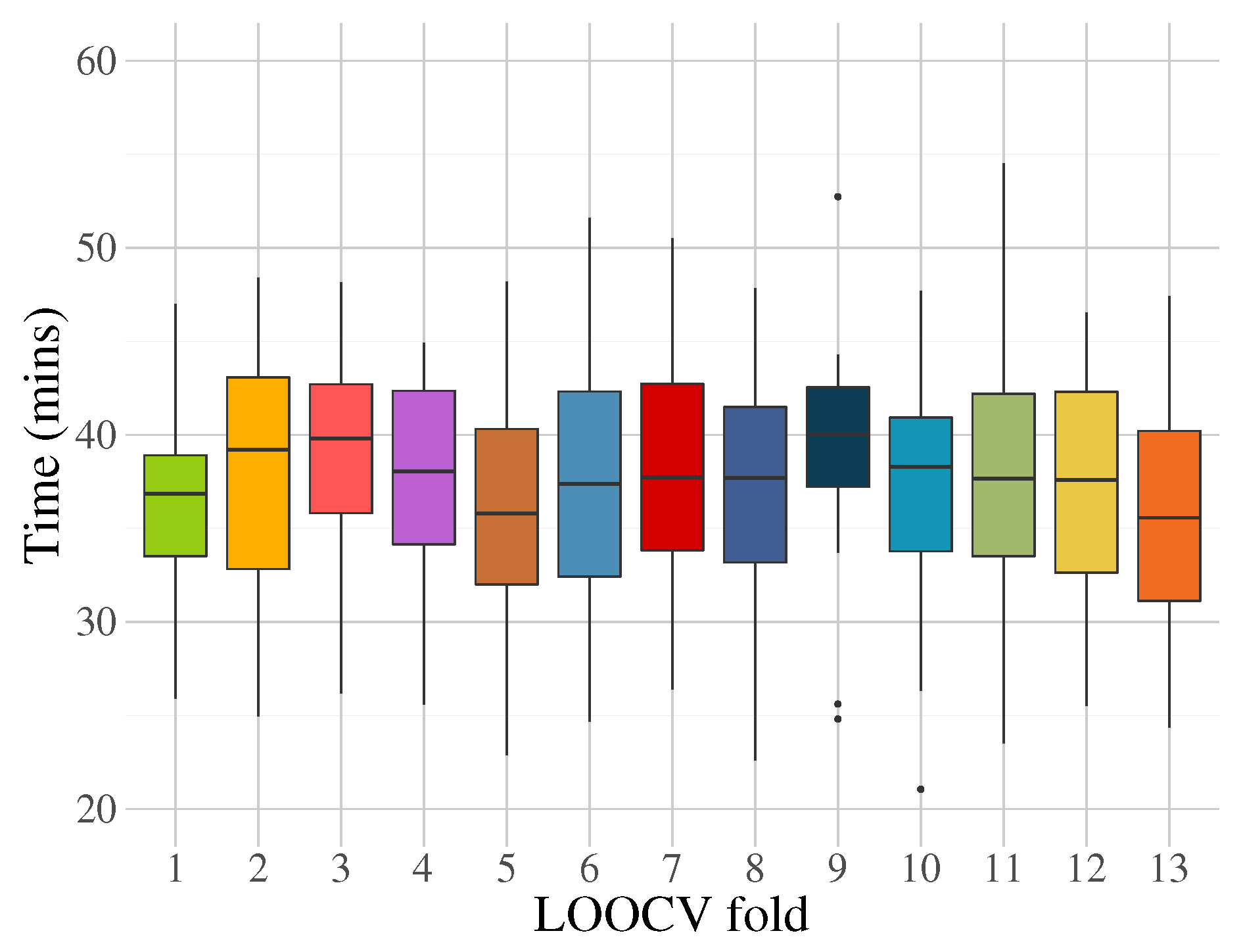
From a different angle, the computational cost in terms of execution time is shown in Figure 19, which indicates a mean of 36 mins for the system to compute a training model. Although the costs can be seen as high compared with other statistical methods, the focus of this implementation is not to achieve small numbers during the training phase, but rather during the testing phase, in which the system accomplishes classification in milliseconds.
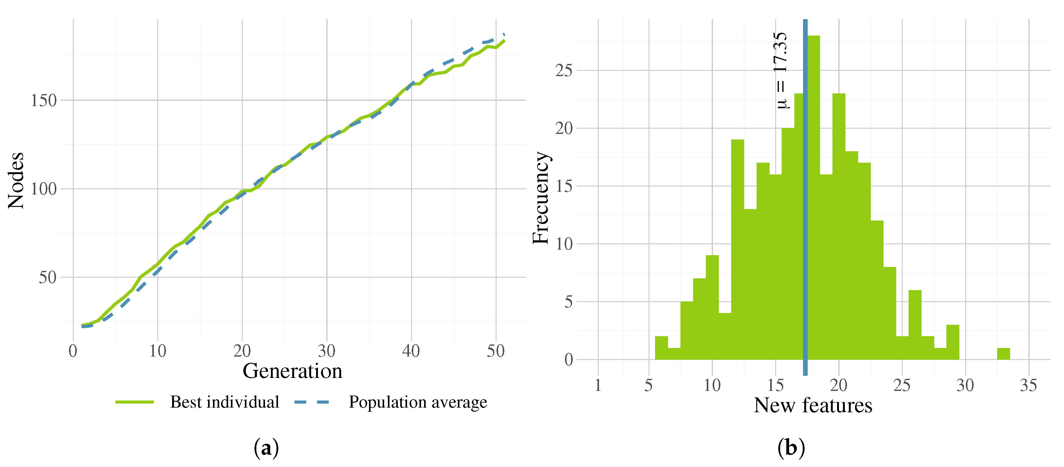
Moreover, if we consider solution sizes in FEGP, shown in Figure 20a (plot lines represents the mean of 13 medians over 30 runs), solutions grow almost linearly during the search. This is a common behavior in GP with tree representations, where the increase of solution size is a product of fitness improvement [51] through the search operators. A side effect of this phenomenon is that sometimes fitness becomes stagnated with unnecessary growth of trees, referred to as bloat [63]. However, in our experiments with a relatively small number of generations for the search, FEGP does not exhibit any bloat, that is, the increase in solution size is always accompanied by a steady improvement in fitness. This was possible due to the regularized fitness measure employed by FEGP.
The increase of solution sizes also means that there is an increase in the number of newly created features, the depth in the tree structure, or both. Specifically, we can see the frequency histogram for all runs and folds in Figure 20b, which show a nearly normal distribution. All individuals were started with three features at the beginning of the runs. The evolved models produced a minimum of six and a maximum of 33 new features, with an average of 17.35.
As mentioned earlier in Section 3, there is an inherent flexibility in terms of the classifier selection after using the FEGP. Therefore, additional classifiers were evaluated: Tree Bagger (TB), Random Forests (https://github.com/ajaiantilal/randomforest-matlab) [64] (RF), k-NN, and SVM. All of them produce non-linear decision functions, as opposed to the relatively simpler LDA. With the exception of RF, all classifiers are based on their MATLAB implementations. The hyperparameters were optimized using a bayesian approach, and are shown in Table 5.
The classification accuracies are summarized in Table 6, including the specificity, recall, and F-score metrics per class. A one-way Analysis of Variance (ANOVA) was performed among the classifiers to estimate statistical significance on the null hypothesis that samples belong to the same distribution. Correlating the results from Table 6, Figure 17 and Figure 18 we can deduce that for this particular problem, more complex classifiers do not produce better accuracies for unseen data; rather, they all over-fit. One reason for this is that most of these algorithms perform accurately if there are enough data to learn; however, for the case of under-sampled data, sometimes, simpler models produce better results. The simpler assumptions of LDA (which, in this case, are actually infringed upon: Class distributions are not normal, nor do they share the same covariance) help to relax the model and behave better as a generalization method.
6. Conclusions and Future Work
This paper proposes a new system for the classification of two mental states based on EEG recordings, with the introduction of a novel GP algorithm that performs as a feature extraction method. The proposed system involves several functional blocks: acquisition of signals, pre-processing, feature extraction, and classification. This work is the first to use a GP-based algorithm for feature extraction for the identification of mental states (specifically, normal and relaxed states).
A reference system was implemented based on our previous work [9], which produced competitive results among similar research works in this domain. Nevertheless, the proposed system outperformed our previous results by further exploiting the separability of classes using evolved transformation models. Certainly, apart from the appropriate choice of the classifier, one of the most important blocks in these types of systems is the feature extraction process, where the pattern recognition of the underlying data is performed.
Evidence found during experimentation allowed us to provide some insights in the following directions. First, the FEGP algorithm in a wrapper scheme produced improved performance compared to the system with just CSP, reaching a classification accuracy of 78.8% for unseen data. Certainly, any system could efficiently benefit from the hybridization of different tools to achieve competitive results. A sole technique usually cannot tackle such a complex problem. Second, the proposed genetic operators allow us to evolve transformation models with good testing performance. Third, the unique fitness function steered the search toward solutions that avoided over-fitting in most of the cases. Fourth, the sizes of the evolved solutions are relatively small in terms of the number of new features and the number of nodes per subtree, resulting in faster execution times during the testing phase. Moreover, in our tests, FEGP was not affected by bloat [63]. Fifth, although from the system design point of view, the classifier can be interchanged, other classifiers did not produce better results compared with LDA. Nevertheless, when examining the whole scenario, we can state that most of the shortcomings were derived from the underlying data properties. In this case, we could opt for three options—increasing the system’s complexity by incorporating an additional processing step and helping reduce further issues like over-fitting, using adaptive classifiers, or increasing the number of EEG recordings. In all of the circumstances, we can foresee applications of the FEGP outside of this domain, that is, by merely adjusting the fitness function, it can be used in any data transformation scenario.
There are several aspects to consider in future work. One is the introduction of feature selection into the system; ultimately, channel reduction is very important for any real-world scenario, mainly for practical reasons. It is also of our interest to increase the number of mental states in future research. Although we emphasize the benefits of the proposed FEGP algorithm in this work, the exploration of different tools in pre-processing and post-processing is also important. Moreover, we do not express by any means that the FEGP algorithm in conjunction with CSP is the best option, but it is rather a choice that proved to be very competitive in this domain.
It is well researched that simple algorithms like CSP are not capable of performing well with complex brain tasks, and there is a limit where the balance between simplicity and practicality ends. As the computer power increases, the need for simpler methods is not necessarily a wanted goal if the results do not improve. The incorporation of GP into the development of efficient BCI systems can be seen as a viable direction in terms of capacity to find new patterns hidden in EEG data. Although GP, like many other machine learning algorithms, has a costly training phase, the testing phase is rather simpler and more efficient, making it quite useful for BCI systems.
Another aspect is the improvement of the FEGP algorithm itself. Further investigation is required to study the evolution behavior; there are still open questions: What is the relationship between the number of features and the efficiency of individual subtrees? Is there a way to fully avoid bloat in longer searches? Are there better genetic operators that allow one to search more efficiently? In our previous works, by implementing a type of local search into GP, we achieved better results in regression [65] and classification problems [66], suggesting that GP generally benefits from the hybridization of search operators. This encourages us to extend these approaches into this domain.
Despite mentioning computational costs just in terms of execution time along the presentation of this work, which, at the moment, is considered as an off-line methodology, it is important to reduce the algorithm’s complexity and, at the same time, increase accuracy. In future work, a full study will be done in balancing the system’s consumed resources and efficiency by using intrinsic parallel implementations, such as Graphics Processing Units (GPU) or Field-Programmable Gate Arrays (FPGA).
Author Contributions
Conceptualization, E.Z.-F. and L.T.; methodology, E.Z.-F. and P.L.; software, E.Z.-F.; validation, L.T., P.L., and F.F.-A.; formal analysis, E.Z.-F. and P.L.; data curation, F.F.-A.; writing—original draft preparation, E.Z.-F.; writing—review and editing, E.Z.-F., L.T., and P.L.; funding acquisition, L.T. and P.L. All authors have read and agreed to the published version of the manuscript.
Funding
Funding for this work was provided by CONACYT (Mexico) Basic Science Research Project No. 178323, the FP7-Marie Curie-IRSES 2013 European Commission program through project ACoBSEC with contract No. 612689, TECNM with contract No. 8027.20-P, and CONACYT project FC-2015-2/944 “Aprendizaje evolutivo a gran escala”. Finally, the first author was supported by CONACYT scholarship No. 294213.
Conflicts of Interest
The authors declare no conflict of interest. The funders had no role in the design of the study; in the collection, analyses, or interpretation of data; in the writing of the manuscript, or in the decision to publish the results.
References
- Alhola, P.; Plo-Kantola, P. Sleep deprivation: Impact on cognitive performance. Neuropsychiatr. Dis. Treat. 2007, 3, 553–567. [Google Scholar]
- Schmidt, E.; Kincses, W.; Schrauf, M. Assessing driver’s vigilance state during monotonous driving. In Proceedings of the Fourth International Driving Symposium on Human Factors in Driver Assessment, Training and Vehicle Design, Stevenson, Washington, DC, USA, 10 October 2007; pp. 138–145. [Google Scholar]
- Selye, H. The Stress Syndrome. Am. J. Nurs. 1965, 65, 97–99. [Google Scholar]
- Baars, B. A Cognitive Theory of Consciousness; Cambridge University Press: Cambridge, UK, 1988. [Google Scholar]
- Laureys, S. The neural correlate of (un)awareness: Lessons from the vegetative state. Trends Cogn. Sci. 2005, 9, 556–559. [Google Scholar] [CrossRef] [PubMed]
- Prashant, P.; Joshi, A.; Gandhi, V. Brain computer interface: A review. In Proceedings of the 2015 5th Nirma University International Conference on Engineering (NUiCONE), Ahmedabad, India, 25 May 2015; Volume 74, pp. 1–6. [Google Scholar]
- Myrden, A.; Chau, T. Effects of user mental state on EEG-BCI performance. Front. Hum. Neurosci. 2015, 9, 308. [Google Scholar] [CrossRef] [PubMed] [Green Version]
- Siuly, S.; Li, Y.; Zhang, Y. EEG Signal Analysis and Classification: Techniques and Applications; Health Information Science, Springer International Publishing: Cham, Switzerland, 2017. [Google Scholar]
- Vézard, L.; Legrand, P.; Chavent, M.; Faïta-Aïnseba, F.; Trujillo, L. EEG classification for the detection of mental states. Appl. Soft Comput. 2015, 32, 113–131. [Google Scholar] [CrossRef]
- Muñoz, L.; Silva, S.; Trujillo, L. M3GP—Multiclass Classification with GP. In Genetic Programming, Proceedings of the 18th European Conference, EuroGP 2015, Copenhagen, Denmark, 8–10 April 2015; Springer International Publishing: Cham, Switzerland, 2015; pp. 78–91. [Google Scholar]
- Woodman, G.F. A brief introduction to the use of event-related potentials (ERPs) in studies of perception and attention. Atten. Percept. Psychophysiol. 2010, 72, 1–29. [Google Scholar]
- Nicolas-Alonso, L.F.; Gomez-Gil, J. Brain computer interfaces, a review. Sensors 2012, 12, 1211–1279. [Google Scholar] [CrossRef]
- Amiri, S.; Fazel-rezai, R.; Asadpour, V. A Review of Hybrid Brain-Computer Interface Systems. Adv. -Hum.-Comput. Interact. - Spec. Issue Using Brain Waves Control. Comput. Mach. 2013, 1–8. [Google Scholar] [CrossRef]
- Gupta, A.; Agrawal, R.K.; Kaur, B. Performance enhancement of mental task classification using EEG signal: A study of multivariate feature selection methods. Soft Comput. 2015, 19, 2799–2812. [Google Scholar] [CrossRef]
- Trejo, L.J.; Kubitz, K.; Rosipal, R.; Kochavi, R.L.; Montgomery, L.D. EEG-Based Estimation and Classification of Mental Fatigue. Psychology 2015, 6, 572–589. [Google Scholar] [CrossRef] [Green Version]
- Zarjam, P.; Epps, J.; Lovell, N.H. Beyond Subjective Self-Rating: EEG Signal Classification of Cognitive Workload. IEEE Trans. Auton. Ment. Dev. 2015, 7, 301–310. [Google Scholar] [CrossRef]
- Garcés Correa, A.; Orosco, L.; Laciar, E. Automatic detection of drowsiness in EEG records based on multimodal analysis. Med. Eng. Phys. 2014, 36, 244–249. [Google Scholar] [CrossRef] [PubMed]
- Hariharan, M.; Vijean, V.; Sindhu, R.; Divakar, P.; Saidatul, A.; Yaacob, S. Classification of mental tasks using stockwell transform. Comput. Electr. Eng. 2014, 40, 1741–1749. [Google Scholar] [CrossRef]
- Mallikarjun, H.M.; Suresh, H.N.; Manimegalai, P. Mental State Recognition by using Brain Waves. Indian J. Sci. Technol. 2016, 9, 2–6. [Google Scholar] [CrossRef] [Green Version]
- Schultze-Kraft, M.; Dähne, S.; Gugler, M.; Curio, G.; Blankertz, B. Unsupervised classification of operator workload from brain signals. J. Neural Eng. 2016, 13, 036008. [Google Scholar] [CrossRef] [Green Version]
- Wu, W.; Chen, Z.; Gao, X.; Li, Y.; Brown, E.N.; Gao, S. Probabilistic common spatial patterns for multichannel EEG analysis. IEEE Trans. Pattern Anal. Mach. Intell. 2015, 37, 639–653. [Google Scholar] [CrossRef]
- Arvaneh, M.; Guan, C.; Ang, K.K.; Ward, T.E.; Chua, K.S.; Kuah, C.W.K.; Ephraim Joseph, G.J.; Phua, K.S.; Wang, C. Facilitating motor imagery-based brain–computer interface for stroke patients using passive movement. Neural Comput. Appl. 2017, 28, 3259–3272. [Google Scholar] [CrossRef] [Green Version]
- Hajinoroozi, M.; Mao, Z.; Huang, Y. Prediction of driver’s drowsy and alert states from EEG signals with deep learning. In Proceedings of the 2015 IEEE 6th International Workshop on Computational Advances in Multi-Sensor Adaptive Processing, CAMSAP 2015, Cancun, Mexico, 13–16 December 2015; pp. 493–496. [Google Scholar]
- Saidatul, A.; Paulraj, S.Y. Mental Stress Level Classification Using Eigenvector Features and Principal Component Analysis. Commun. Inf. Sci. Manag. Eng. 2013, 3, 254–261. [Google Scholar]
- Guo, L.; Rivero, D.; Dorado, J.; Munteanu, C.R.; Pazos, A. Automatic feature extraction using genetic programming: An application to epileptic EEG classification. Expert Syst. Appl. 2011, 38, 10425–10436. [Google Scholar] [CrossRef]
- Berek, P.; Prilepok, M.; Platos, J.; Snasel, V. Classification of EEG Signals Using Vector Quantization. In International Conference on Artificial Intelligence and Soft Computing; Springer: Zakopane, Poland, 2014; pp. 107–118. [Google Scholar]
- Shen, K.Q.; Li, X.P.; Ong, C.J.; Shao, S.Y.; Wilder-Smith, E.P.V. EEG-based mental fatigue measurement using multi-class support vector machines with confidence estimate. Clin. Neurophysiol. 2008, 119, 1524–1533. [Google Scholar] [CrossRef]
- Khasnobish, A.; Konar, A.; Tibarewala, D.N. Object Shape Recognition from EEG Signals during Tactile and Visual Exploration. In International Conference on Pattern Recognition and Machine Intelligence; Springer: Kolkata, India, 2013; pp. 459–464. [Google Scholar]
- Vézard, L.; Chavent, M.; Legrand, P.; Faïta-Aïnseba, F.; Trujillo, L. Detecting mental states of alertness with genetic algorithm variable selection. In Proceedings of the 2013 IEEE Congress on Evolutionary Computation, CEC 2013, Cancun, Mexico, 20–23 June 2013; pp. 1247–1254. [Google Scholar]
- Fang, C.; Li, H.; Ma, L. EEG Signal Classification Using the Event-Related Coherence and Genetic Algorithm. In Advances in Brain Inspired Cognitive Systems; Springer: Beijing, China, 2013; pp. 92–100. [Google Scholar]
- Rezaee, A. Applying Genetic Algorithm to EEG Signals for Feature Reduction in Mental Task Classification. Int. J. Smart Electr. Eng. 2016, 5, 4–7. [Google Scholar]
- Hongxia, L.; Hongxi, D.; Jian, L.; Shuicheng, T. Research on the application of the improved genetic algorithm in the electroencephalogram-based mental workload evaluation for miners. J. Algorithms Comput. Technol. 2016, 10, 1–10. [Google Scholar] [CrossRef]
- Orriols-Puig, A.; Casillas, J.; Bernadó-Mansilla, E. A Comparative Study of Several Genetic-Based Supervised Learning Systems. In Learning Classifier Systems in Data Mining; Springer: Berlin, Heidelberg, 2008; Volume 125, pp. 205–230. [Google Scholar]
- Erguzel, T.T.; Ozekes, S.; Gultekin, S.; Tarhan, N. Ant colony optimization based feature selection method for QEEG data classification. Psychiatry Investig. 2014, 11, 243–250. [Google Scholar] [CrossRef] [PubMed] [Green Version]
- Mirvaziri, H.; Mobarakeh, Z.S. Improvement of EEG-based motor imagery classification using ring topology-based particle swarm optimization. Biomed. Signal Process. Control. 2017, 32, 69–75. [Google Scholar] [CrossRef]
- Hassani, K.; Lee, W.s. An Incremental Framework for Classification of EEG Signals Using Quantum Particle Swarm Optimization. In IEEE International Conference on Computational Intelligence and Virtual Environments for Measurement Systems and Applications (CIVEMSA); IEEE: Ottawa, ON, Canada, 2014; pp. 40–45. [Google Scholar]
- Bhardwaj, A.; Tiwari, A.; Varma, M.V.; Krishna, M.R. Classification of EEG signals using a novel genetic programming approach. In Proceedings of the 2014 Conference Companion on Genetic and Evolutionary Computation Companion—GECCO Comp ’14, Vancouver, BC, Canada, 12–16 July 2014; pp. 1297–1304. [Google Scholar]
- Bhardwaj, A.; Tiwari, A.; Krishna, R.; Varma, V. A novel genetic programming approach for epileptic seizure detection. Comput. Methods Programs Biomed. 2016, 124, 2–18. [Google Scholar] [CrossRef]
- Fernández-Blanco, E.; Rivero, D.; Gestal, M.; Dorado, J. Classification of signals by means of Genetic Programming. Soft Comput. 2013, 17, 1929–1937. [Google Scholar] [CrossRef]
- Sotelo, A.; Guijarro, E.; Trujillo, L.; Coria, L.N.; Martínez, Y. Identification of epilepsy stages from {ECoG} using genetic programming classifiers. Comput. Biol. Med. 2013, 43, 1713–1723. [Google Scholar] [CrossRef]
- Lin, J.Y.; Ke, H.R.; Chien, B.C.; Yang, W.P. Designing a classifier by a layered multi-population genetic programming approach. Pattern Recognit. 2007, 40, 2211–2225. [Google Scholar] [CrossRef]
- Chien, B.C.; Lin, J.Y.; Yang, W.P. Learning effective classifiers with -value measure based on genetic programming. Pattern Recognit. 2004, 37, 1957–1972. [Google Scholar] [CrossRef]
- Smart, O.; Firpi, H.; Vachtsevanos, G. Genetic programming of conventional features to detect seizure precursors. Eng. Appl. Artif. Intell. 2007, 20, 1070–1085. [Google Scholar] [CrossRef] [Green Version]
- Sabeti, M.; Katebi, S.; Boostani, R. Entropy and complexity measures for EEG signal classification of schizophrenic and control participants. Artif. Intell. Med. 2009, 47, 263–274. [Google Scholar] [CrossRef] [PubMed]
- Guo, H.; Zhang, Q.; Nandi, A.K. Feature extraction and dimensionality reduction by genetic programming based on the Fisher criterion. Expert Syst. 2008, 25, 444–459. [Google Scholar] [CrossRef]
- Walter, W.G.; Cooper, R.; Aldridge, V.J.; McCallum, W.C.; Winter, A.L. Contingent Negative Variation: An Electric Sign of Sensori-Motor Association and Expectancy in the Human Brain. Nature 1964, 203, 380–384. [Google Scholar] [CrossRef] [PubMed]
- Pfurtscheller, G.; Neuper, C.; Flotzinger, D.; Pregenzer, M. EEG-based discrimination between imagination of right and left hand movement. Electroencephalogr. Clin. Neurophysiol. 1997, 103, 642–651. [Google Scholar] [CrossRef]
- Ramoser, H.; Müller-Gerking, J.; Pfurtscheller, G. Optimal spatial filtering of single trial EEG during imagined hand movement. IEEE Trans. Rehabil. Eng. 2000, 8, 441–446. [Google Scholar] [CrossRef] [PubMed] [Green Version]
- Blankertz, B.; Tomioka, R.; Lemm, S.; Kawanabe, M.; Muller, K.r. Optimizing Spatial filters for Robust EEG Single-Trial Analysis. IEEE Signal Process. Mag. 2008, 25, 41–56. [Google Scholar] [CrossRef]
- Duda, R.O.; Hart, P.E.; Stork, D.G. Pattern Classification, 2nd ed.; Wiley-Interscience: New York, NY, USA, 2000. [Google Scholar]
- Koza, J.R. Genetic Programming: On the Programming of Computers by Means of Natural Selection; MIT Press: Cambridge, MA, USA, 1992. [Google Scholar]
- Goldberg, D.E. Genetic Algorithms in Search, Optimization and Machine Learning, 1st ed.; Addison-Wesley Longman Publishing Co., Inc.: Boston, MA, USA, 1989. [Google Scholar]
- Koza, J.R. Human-competitive results produced by genetic programming. Genet. Program. Evolvable Mach. 2010, 11, 251–284. [Google Scholar] [CrossRef] [Green Version]
- O’Neill, M.; Vanneschi, L.; Gustafson, S.; Banzhaf, W. Open issues in Genetic Programming. Genet. Program. Evolvable Mach. 2010, 11, 339–363. [Google Scholar] [CrossRef] [Green Version]
- Hastie, T.; Tibshirani, R.; Friedman, J.; Hastie, T.; Friedman, J.; Tibshirani, R. The Elements of Statistical Learning: Data Mining, Inference, and Prediction; Springer: Berlin/Heidelberg, Germany, 2009; Volume 2. [Google Scholar]
- Cawley, G.C.; Talbot, N.L.C. On Over-fitting in Model Selection and Subsequent Selection Bias in Performance Evaluation. J. Mach. Learn. Res. 2010, 11, 2079–2107. [Google Scholar]
- Naredo, E.; Trujillo, L.; Legrand, P.; Silva, S.; Muñoz, L. Evolving genetic programming classifiers with novelty search. Inf. Sci. 2016, 369, 347–367. [Google Scholar] [CrossRef]
- Firpi, H.; Goodman, E.; Echauz, J. On prediction of epileptic seizures by means of genetic programming artificial features. Ann. Biomed. Eng. 2006, 34, 515–529. [Google Scholar] [CrossRef] [PubMed]
- Poli, R.; Salvaris, M.; Cinel, C. Evolution of a brain-computer interface mouse via genetic programming. Lect. Notes Comput. Sci. (Including Subser. Lect. Notes Artif. Intell. Lect. Notes Bioinf.) 2011, 6621 LNCS, 203–214. [Google Scholar]
- Tuson, A.; Ross, P. Adapting operator settings in genetic algorithms. Evol. Comput. 1998, 6, 161–184. [Google Scholar] [CrossRef] [PubMed] [Green Version]
- Ho, T.K.; Basu, M. Complexity measures of supervised classification problems. IEEE Trans. Pattern Anal. Mach. Intell. 2002, 24, 289–300. [Google Scholar]
- Silva, S.; Almeida, J. GPLAB—A genetic programming toolbox for MATLAB. In Proceedings of the Nordic MATLAB Conference, Copenhagen, Denmark, 21–22 October 2003; pp. 273–278. [Google Scholar]
- Silva, S.; Costa, E. Dynamic limits for bloat control in genetic programming and a review of past and current bloat theories. Genet. Program. Evolvable Mach. 2009, 10, 141–179. [Google Scholar] [CrossRef]
- Jaiantilal, A. RF Matlab Interface, Version 0.02, Github. Available online: https://github.com/ajaiantilal/randomforest-matlab (accessed on 22 August 2020).
- Z-Flores, E.; Trujillo, L.; Schütze, O.; Legrand, P. Evaluating the Effects of Local Search in Genetic Programming. In EVOLVE—A Bridge between Probability, Set Oriented Numerics, and Evolutionary Computation V; Springer International Publishing: Cham, Switzerland, 2014; Volume 288, pp. 213–228. [Google Scholar]
- Z-Flores, E.; Trujillo, L.; Schütze, O.; Legrand, P. A Local Search Approach to Genetic Programming for Binary Classification. In Proceedings of the 2015 on Genetic and Evolutionary Computation Conference-GECCO ’15, Madrid, Spain, 11–15 July 2015; pp. 1151–1158. [Google Scholar]
Figure 1.
Methodology of the reference system.

Figure 2.
Frequency response for the Butterworth filter used in this work.

Figure 3.
Classification performance for the reference system.

Figure 4.
Methodology for the proposed enhanced system.

Figure 5.
Genetic Programming (GP) flowchart in a nutshell.

Figure 6.
Block diagram for the proposed Augmented Feature Extraction with Genetic Programming (FEGP).
Figure 6.
Block diagram for the proposed Augmented Feature Extraction with Genetic Programming (FEGP).

Figure 7.
FEGP individual representation.

Figure 8.
FEGP inter-crossover, swapping subtrees between different individuals. is the local fitness; the crossover points are chosen from the subtrees with .
Figure 8.
FEGP inter-crossover, swapping subtrees between different individuals. is the local fitness; the crossover points are chosen from the subtrees with .

Figure 9.
FEGP intra-crossover, swapping subtrees within the same individual.

Figure 10.
FEGP inter-individual feature crossover.

Figure 11.
FEGP feature insertion mutation. A new randomly created subtree is added to a tree with r subtrees.
Figure 11.
FEGP feature insertion mutation. A new randomly created subtree is added to a tree with r subtrees.

Figure 12.
Operator probabilities through the search.

Figure 13.
Class variance penalization, where (a) corresponds to the tree output—in this example are new features—and (b) corresponds to the data modification with a larger distribution variance used to compute the global fitness.
Figure 13.
Class variance penalization, where (a) corresponds to the tree output—in this example are new features—and (b) corresponds to the data modification with a larger distribution variance used to compute the global fitness.

Figure 14.
Training and testing performance for both the reference system and the proposed enhanced system for each Leave-One-Out Cross-Validation (LOOCV) fold. Mean values for all folds are shown.
Figure 14.
Training and testing performance for both the reference system and the proposed enhanced system for each Leave-One-Out Cross-Validation (LOOCV) fold. Mean values for all folds are shown.

Figure 15.
Box plots of the enhanced system performance for 30 runs per fold, where (a) corresponds to the classification accuracy for the training partition and (b) is homologous for the testing partition.
Figure 15.
Box plots of the enhanced system performance for 30 runs per fold, where (a) corresponds to the classification accuracy for the training partition and (b) is homologous for the testing partition.

Figure 16.
Linear Discriminant Analysis (LDA) classification accuracy for the evolution of fitness. The accuracy plots show the history of LDA accuracy calculated over the best individual per fold; this represents the median over 30 independent runs. The fitness plot shows the evolution of fitness from the best individual representing the mean of the 13 (folds) medians over 30 runs by (a) using training data and (b) using testing data.

Figure 17.
The first two components from Principal Component Analysis (PCA) corresponding to fold 4 in the LOOCV. Plot (a) is the class distribution for the raw data; (b) after the Common Spatial Pattern (CSP); and (c) after the best transformation found by FEGP. Classification accuracy is 82.8% for training and 99.1% for testing.

Figure 18.
The first two components from PCA corresponding to fold 8 in the LOOCV. Plot (a) is the class distribution for the raw data; (b) after the CSP; and (c) after the best transformation found by FEGP. Classification accuracy is 81.4% for training and 44.1% for testing.
Figure 18.
The first two components from PCA corresponding to fold 8 in the LOOCV. Plot (a) is the class distribution for the raw data; (b) after the CSP; and (c) after the best transformation found by FEGP. Classification accuracy is 81.4% for training and 44.1% for testing.

Figure 19.
Execution time for FEGP implementation during the training phase for each LOOCV fold using the experimental setup.
Figure 19.
Execution time for FEGP implementation during the training phase for each LOOCV fold using the experimental setup.

Figure 20.
(a) Evolution of best individual and population average sizes, showing the mean of 13 medians over 30 runs. (b) Frequency histogram of the number of new features produced by the FEGP algorithm.
Figure 20.
(a) Evolution of best individual and population average sizes, showing the mean of 13 medians over 30 runs. (b) Frequency histogram of the number of new features produced by the FEGP algorithm.


Table 1.
FEGP parameters used in the experiments.
| Parameter | Value | Comments |
|---|---|---|
| Generations | 50 | If the max depth for the evolved trees is relatively small, then more generations are not needed, since the solution size is restricted and the overall search stagnates. |
| Population size | 100 | A small population was found to be sufficient to evolve good solutions with larger populations, reaching the same performance. |
| Population initialization | Full | Since the search space can be huge, very small individuals are not beneficial to quickly explore the solution space. |
| Population init max depth | 5 levels | A good compromise between structure diversity and complexity. |
| Initial features | 3 | Variable r. |
| Search operators | Inter-crossover, inter-feature crossover, intra-crossover, mutation, feature insertion, feature removal | |
| Initial probabilities for search operators | 0.2, 0.2, 0.2, 0.05, 0.15, 0.1 | Each value corresponds to each operator in the same order as the above list. |
| Delta values for decay function | 0.2 | This only applies to the inter-crossover operator. |
| Function set | +,−,×,/,log,cos,sin, tan,√,abs | |
| Terminal set | random [0,1], input features | |
| Max depth level | 20 | Since individuals can have several features, big values for the allowed depth are not desired. If a child tree is above this limit after the genetic operation, then it is discarded and a reproduction operation is performed instead. |
| Selection | Tournament, size 5 | A small tournament size provides a richer diversity in the population. |
| Elitism | Only best individual survives | Assures that the best solution is not lost from generation to generation. |
Table 2.
FEGP training and testing performance for each LOOCV fold in terms of its accuracy (%), kappa coefficient (), and p-values for kappa statistical tests. Bold values indicate that observed agreement between true and predicted labels is not accidental.
Table 2.
FEGP training and testing performance for each LOOCV fold in terms of its accuracy (%), kappa coefficient (), and p-values for kappa statistical tests. Bold values indicate that observed agreement between true and predicted labels is not accidental.
| 1 | 2 | 3 | 4 | 5 | 6 | 7 | 8 | 9 | 10 | 11 | 12 | 13 | ||
|---|---|---|---|---|---|---|---|---|---|---|---|---|---|---|
| Training | Accuracy | 83.5 | 81.6 | 86 | 81.5 | 83 | 82.5 | 79.3 | 84.9 | 81.5 | 80.7 | 81.9 | 83.5 | 75.8 |
| 0.70 | 0.68 | 0.77 | 0.63 | 0.72 | 0.56 | 0.72 | 0.77 | 0.64 | 0.49 | 0.77 | 0.69 | 0.63 | ||
| p-value | 0.0000 | 0.0000 | 0.0000 | 0.0000 | 0.0000 | 0.0000 | 0.0000 | 0.0000 | 0.0000 | 0.0000 | 0.0000 | 0.0000 | 0.0000 | |
| Testing | Accuracy | 82.9 | 82.7 | 58 | 96.5 | 95 | 60.2 | 89.3 | 46 | 82.8 | 87.4 | 91.2 | 63 | 88.6 |
| 0.70 | 0.65 | 0.16 | 0.90 | 0.88 | 0.30 | 0.79 | 0.01 | 0.72 | 0.81 | 0.78 | 0.24 | 0.75 | ||
| p-value | 0.0000 | 0.0000 | 0.3346 | 0.0000 | 0.0000 | 0.0023 | 0.0000 | 0.9702 | 0.0000 | 0.0000 | 0.0000 | 0.1379 | 0.0000 |
Table 3.
Statistical pairwise tests corresponding to the training performance. The upper triangular matrix encloses the p-values for a two-sample Kolmogorov–Smirnov test and the lower triangular matrix consists of the p-values for a Wilcoxon rank sum test. Bold values indicate that the null hypothesis is rejected at the significance level for both tests.
| 1 | 2 | 3 | 4 | 5 | 6 | 7 | 8 | 9 | 10 | 11 | 12 | 13 | |
|---|---|---|---|---|---|---|---|---|---|---|---|---|---|
| 1 | - | 0.0011 | 0.0000 | 0.0108 | 0.3038 | 0.0706 | 0.0000 | 0.0108 | 0.0003 | 0.0108 | 0.0290 | 0.3038 | 0.0000 |
| 2 | 0.0168 | - | 0.0000 | 0.5309 | 0.0706 | 0.3038 | 0.0706 | 0.0108 | 0.9728 | 0.9728 | 0.1545 | 0.0290 | 0.0001 |
| 3 | 0.0001 | 0.0000 | - | 0.0000 | 0.0000 | 0.0036 | 0.0000 | 0.0108 | 0.0000 | 0.0001 | 0.0003 | 0.0036 | 0.0000 |
| 4 | 0.0206 | 0.6327 | 0.0000 | - | 0.1545 | 0.3038 | 0.0011 | 0.0036 | 0.7974 | 0.5309 | 0.7974 | 0.0290 | 0.0000 |
| 5 | 0.5799 | 0.0442 | 0.0000 | 0.0741 | - | 0.3038 | 0.0001 | 0.0290 | 0.1545 | 0.0290 | 0.5309 | 0.5309 | 0.0000 |
| 6 | 0.6326 | 0.1589 | 0.0103 | 0.2683 | 0.8602 | - | 0.0036 | 0.3038 | 0.3038 | 0.5309 | 0.7974 | 0.5309 | 0.0000 |
| 7 | 0.0001 | 0.1020 | 0.0000 | 0.0048 | 0.0000 | 0.0021 | - | 0.0003 | 0.0706 | 0.0706 | 0.0003 | 0.0003 | 0.0003 |
| 8 | 0.2370 | 0.0180 | 0.0030 | 0.0206 | 0.1445 | 0.6689 | 0.0005 | - | 0.0036 | 0.0290 | 0.0706 | 0.5309 | 0.0000 |
| 9 | 0.0071 | 0.9198 | 0.0000 | 0.4970 | 0.0221 | 0.1130 | 0.0741 | 0.0111 | - | 0.9728 | 0.1545 | 0.0108 | 0.0001 |
| 10 | 0.0871 | 0.6873 | 0.0000 | 0.8405 | 0.0782 | 0.2370 | 0.0441 | 0.0469 | 0.6326 | - | 0.0706 | 0.1545 | 0.0000 |
| 11 | 0.2176 | 0.1908 | 0.0004 | 0.5973 | 0.4657 | 0.6507 | 0.0005 | 0.2576 | 0.1743 | 0.2177 | - | 0.3038 | 0.0000 |
| 12 | 0.6689 | 0.0559 | 0.0046 | 0.0497 | 0.4063 | 0.8014 | 0.0008 | 0.7820 | 0.0268 | 0.1445 | 0.3023 | - | 0.0000 |
| 13 | 0.0000 | 0.0000 | 0.0000 | 0.0000 | 0.0000 | 0.0000 | 0.0004 | 0.0000 | 0.0000 | 0.0000 | 0.0000 | 0.0000 | - |
Table 4.
Statistical pairwise tests corresponding to the testing performance. The upper triangular matrix encloses the p-values for a two-sample Kolmogorov–Smirnov test, and the lower triangular matrix consists of the p-values for a Wilcoxon rank sum test. Bold values indicate that the null hypothesis is rejected at the significance level for both tests.
| 1 | 2 | 3 | 4 | 5 | 6 | 7 | 8 | 9 | 10 | 11 | 12 | 13 | |
|---|---|---|---|---|---|---|---|---|---|---|---|---|---|
| 1 | - | 0.5309 | 0.0000 | 0.0000 | 0.0000 | 0.0000 | 0.0000 | 0.0000 | 0.0290 | 0.0000 | 0.0000 | 0.0000 | 0.0000 |
| 2 | 0.4484 | - | 0.0000 | 0.0000 | 0.0000 | 0.0000 | 0.0000 | 0.0000 | 0.3038 | 0.0000 | 0.0000 | 0.0000 | 0.0000 |
| 3 | 0.0000 | 0.0000 | - | 0.0000 | 0.0000 | 0.0290 | 0.0000 | 0.0000 | 0.0000 | 0.0000 | 0.0000 | 0.0000 | 0.0000 |
| 4 | 0.0000 | 0.0000 | 0.0000 | - | 0.1545 | 0.0000 | 0.0000 | 0.0000 | 0.0000 | 0.0000 | 0.0001 | 0.0000 | 0.0000 |
| 5 | 0.0000 | 0.0000 | 0.0000 | 0.0521 | - | 0.0000 | 0.0000 | 0.0000 | 0.0000 | 0.0000 | 0.0036 | 0.0000 | 0.0000 |
| 6 | 0.0000 | 0.0000 | 0.0284 | 0.0000 | 0.0000 | - | 0.0000 | 0.0000 | 0.0000 | 0.0000 | 0.0000 | 0.0706 | 0.0000 |
| 7 | 0.0000 | 0.0000 | 0.0000 | 0.0000 | 0.0000 | 0.0000 | - | 0.0000 | 0.0000 | 0.0290 | 0.0036 | 0.0000 | 0.3038 |
| 8 | 0.0000 | 0.0000 | 0.0000 | 0.0000 | 0.0000 | 0.0000 | 0.0000 | - | 0.0000 | 0.0000 | 0.0000 | 0.0000 | 0.0000 |
| 9 | 0.3501 | 0.8996 | 0.0000 | 0.0000 | 0.0000 | 0.0000 | 0.0000 | 0.0000 | - | 0.0000 | 0.0000 | 0.0000 | 0.0000 |
| 10 | 0.0000 | 0.0000 | 0.0000 | 0.0000 | 0.0000 | 0.0000 | 0.1258 | 0.0000 | 0.0000 | - | 0.0000 | 0.0000 | 0.0706 |
| 11 | 0.0000 | 0.0000 | 0.0000 | 0.0000 | 0.0101 | 0.0000 | 0.0012 | 0.0000 | 0.0000 | 0.0000 | - | 0.0000 | 0.0003 |
| 12 | 0.0000 | 0.0000 | 0.0001 | 0.0000 | 0.0000 | 0.0232 | 0.0000 | 0.0000 | 0.0000 | 0.0000 | 0.0000 | - | 0.0000 |
| 13 | 0.0000 | 0.0000 | 0.0000 | 0.0000 | 0.0000 | 0.0000 | 0.5435 | 0.0000 | 0.0000 | 0.7784 | 0.0007 | 0.0000 | - |
Table 5.
Summary of the parameters and hyperparameters used for the additional classifiers.
| Classifier | Parameter | Value |
|---|---|---|
| Tree Bagger (TB) | Number of trees | 200 |
| Number of observations per leaf | 5 | |
| Number of predictors to sample at each node | 6 | |
| Random Forests (RF) | Number of trees | 300 |
| Minimum node size | 5 | |
| Number of predictors sampled for splitting at each node | 4 | |
| k-Nearest Neighbors (k-NN) | Search method | k-d tree |
| Maximum number of data points in the leaf node | 50 | |
| Number of nearest neighbors | 8 | |
| Distance metric | Manhattan | |
| Distance weighting function | None | |
| Support Vector Machine (SVM) | Kernel function | Gaussian |
| Kernel scale | 56.78 | |
| Kernel offset | 0 | |
| Box constraint | 994.49 | |
| Optimization routine | Sequential minimal optimization |
Table 6.
Classifier performance for the FEGP algorithm. Values for specificity, recall, and F-score represent means over 13 folds; the accuracies also highlight the standard deviation. refers to the normal state and refers to the relaxed state. The last row shows the one-way Analysis of Variance (ANOVA) test between classifiers in terms of the accuracy; bold values indicate that the null hypothesis is rejected at an significance level.
| Name | Training | Testing | |||||||
|---|---|---|---|---|---|---|---|---|---|
| Specificity | Recall | F-Score | Accuracy | Specificity | Recall | F-Score | Accuracy | ||
| LDA | 0.8014 | 0.8201 | 0.8308 | 0.7993 | 0.7684 | 0.7713 | |||
| 0.8201 | 0.8014 | 0.8002 | 0.7684 | 0.7993 | 0.8001 | ||||
| Average | 0.8108 | 0.8108 | 0.8155 | 0.7838 | 0.7838 | 0.7857 | |||
| TB | 1.0000 | 1.0000 | 1.0000 | 0.7552 | 0.7134 | 0.6852 | |||
| 1.0000 | 1.0000 | 1.0000 | 0.7134 | 0.7552 | 0.7203 | ||||
| Average | 1.0000 | 1.0000 | 1.0000 | 0.7343 | 0.7343 | 0.7027 | |||
| RF | 1.0000 | 1.0000 | 1.0000 | 0.7751 | 0.7082 | 0.6795 | |||
| 1.0000 | 1.0000 | 1.0000 | 0.7082 | 0.7751 | 0.7205 | ||||
| Average | 1.0000 | 1.0000 | 1.0000 | 0.7417 | 0.7417 | 0.7000 | |||
| k-NN | 1.0000 | 1.0000 | 1.0000 | 0.6768 | 0.6131 | 0.6118 | |||
| 1.0000 | 1.0000 | 1.0000 | 0.6131 | 0.6768 | 0.6483 | ||||
| Average | 1.0000 | 1.0000 | 1.0000 | 0.6449 | 0.6449 | 0.6300 | |||
| SVM | 0.9627 | 0.9570 | 0.9587 | 0.6533 | 0.6759 | 0.6334 | |||
| 0.9570 | 0.9627 | 0.9607 | 0.6759 | 0.6533 | 0.6232 | ||||
| Average | 0.9598 | 0.9598 | 0.9597 | 0.6646 | 0.6646 | 0.6283 | |||
| p-value | 0.0000 | 0.0687 | |||||||
© 2020 by the authors. Licensee MDPI, Basel, Switzerland. This article is an open access article distributed under the terms and conditions of the Creative Commons Attribution (CC BY) license (http://creativecommons.org/licenses/by/4.0/).
Share and Cite
MDPI and ACS Style
Z-Flores, E.; Trujillo, L.; Legrand, P.; Faïta-Aïnseba, F. EEG Feature Extraction Using Genetic Programming for the Classification of Mental States. Algorithms 2020, 13, 221. https://doi.org/10.3390/a13090221
AMA Style
Z-Flores E, Trujillo L, Legrand P, Faïta-Aïnseba F. EEG Feature Extraction Using Genetic Programming for the Classification of Mental States. Algorithms. 2020; 13(9):221. https://doi.org/10.3390/a13090221
Chicago/Turabian StyleZ-Flores, Emigdio, Leonardo Trujillo, Pierrick Legrand, and Frédérique Faïta-Aïnseba. 2020. "EEG Feature Extraction Using Genetic Programming for the Classification of Mental States" Algorithms 13, no. 9: 221. https://doi.org/10.3390/a13090221
Note that from the first issue of 2016, this journal uses article numbers instead of page numbers. See further details here.