
Towards a Vectorial Approach to Predict Beef Farm Performance


1
Department of Veterinary Sciences, University of Torino, Largo Paolo Braccini 2, 10095 Grugliasco, Italy
2
Associazione Nazionale Allevatori Bovini Razza Piemontese, 12061 Carru, Italy
3
NOVA Information Management School (NOVA IMS), Universidade Nova de Lisboa, Campus de Campolide, 1070-312 Lisboa, Portugal
*
Author to whom correspondence should be addressed.
Appl. Sci. 2022, 12(3), 1137; https://doi.org/10.3390/app12031137
Submission received: 9 December 2021
/
Revised: 9 January 2022
/
Accepted: 16 January 2022
/
Published: 21 January 2022
(This article belongs to the Special Issue Bio-Inspired Computational Techniques: Theory, Methods and Applications)
Abstract
:Accurate livestock management can be achieved by means of predictive models. Critical factors affecting the welfare of intensive beef cattle husbandry systems can be difficult to be detected, and Machine Learning appears as a promising approach to investigate the hundreds of variables and temporal patterns lying in the data. In this article, we explore the use of Genetic Programming (GP) to build a predictive model for the performance of Piemontese beef cattle farms. In particular, we investigate the use of vectorial GP, a recently developed variant of GP, that is particularly suitable to manage data in a vectorial form. The experiments conducted on the data from 2014 to 2018 confirm that vectorial GP can outperform not only the standard version of GP but also a number of state-of-the-art Machine Learning methods, such as k-Nearest Neighbors, Generalized Linear Models, feed-forward Neural Networks, and long- and short-term memory Recurrent Neural Networks, both in terms of accuracy and generalizability. Moreover, the intrinsic ability of GP in performing an automatic feature selection, while generating interpretable predictive models, allows highlighting the main elements influencing the breeding performance.
1. Introduction
A large amount of data are nowadays collected in the livestock sector [1,2,3,4]. It is increasingly common to monitor animals, for greater accuracy in the quantity and quality of information, to achieve economic and environmental sustainability of farms. The breeder must generally deal with animals’ issues, such as their health conditions and social behavior, affecting the quality of the product, the animals’ welfare, and the performance of the farm. The digitization of data collection made it possible to streamline and accelerate the procedures of data collection and processing over time, permitting the registration and consequent elaboration of many additional data, going under the name of Precision Livestock Farming (PLF) [2,5]. The resulting knowledge, processed through mathematical and computational models, may provide the offset of overall incurred costs of the farm, as relevant issues are identified in advance, allowing decisions to be made in time [6,7,8]. The major consequence of a continuous monitoring of animals is a huge amount of data, the so-called “Big Data”, contributing to an increase in the complexity among databases. If, on the one side, the PLF approach aims at a greater “accuracy” in the quantity and quality of information, entailing the development of monitoring systems, on the other side, it must deal with the transformation of big data into meaningful information. The increase in the amount of data requires the introduction of proper data management and prediction techniques. Machine Learning (ML) is based on the availability of large amounts of information and on computing power. Rather than making a priori assumptions and following pre-programmed algorithms, ML allows the system to learn from data. Hence, this field of research is suitable for the management of large datasets, without assuming too specific nor restrictive hypotheses among data [9]. ML is commonly used to predict livestock issues [7,10], such as time of disease events, risk factors for health conditions, failure to complete a production cycle, as well as the genome of complex traits [11]. Despite the biological process being too complex to replace farmers with technology, it still offers more possibilities to save money and to change farmers’ lives, as a more accurate management system can be achieved, leading to a better approach to the genetic potential of today’s livestock species [1,7,8]. Studies have been conducted, based on the application of ML techniques, to model the individual intake of cow feed, optimizing health and fertility, to predict the rumen fermentation pattern from milk fatty acids, which influence the quantity and composition of the milk produced but also the sensorial and technological characteristics of the meat [10,12].
A great variety of studies is available in the milk sector, as opposed to the meat sector, where the use of devices is still moderate. Within the beef cattle sector, it fits the Italian Piemontese, raised in intensive farms mostly concentrated in the Italian region of Piedmont [13,14]. Its preservation is guaranteed by the National Association of Piemontese Cattle Breeders, ANABORAPI in brief. This Association is hence responsible for promoting the breed through the study of the productive, reproductive, and management processes of Piemontese breeding. The direction towards which modern Piemontese breeding aims is the production of calves for fattening. To maximize revenues, it is therefore essential that each dam produces as many calves as possible during her productive career, in full respect of her physiology. The indicator parameter of a cow’s reproductive efficiency is represented by the “calf quota” per cow, derived form the calving interval. If well managed, the current Piemontese cow can produce and raise almost one calf per year, not to mention twin births. The reproductive capacity of the cows that lodge on the farm significantly affects the farmer’s income. Damage derives from the loss of income from the failure to give birth to calves and from the cost of feeding the cows. In this direction, great strides have been made, above all, with regard to the selection of animals capable of giving birth well and calves that are not excessively large but are able to develop excellent growth. These are the aspects that improve the breed’s aptitude for giving birth. Since the process to improve calving ease is slow, it is also necessary to take advantage of all the technical and managerial factors of the herd that can affect the trend of births on the farm. Cow management, in terms of feed and type of housing, a correct choice of mating, the possibility of having a suitable environment where to give birth, and knowledge about birth events, allows the farmer to set the conditions necessary for the optimal performance of this event. It is obvious that, among other things, the calving depends strictly on the fertility of the cow. Among the possible causes of a herd’s fertility reduction, those intrinsic to feeding system, infectious, hygienic-sanitary, or endocrine-gynecological ones and those of environmental nature are of major importance. Not to forget that all stressful conditions, such as uncomfortable housing, insufficient lighting, and crumbling shelters, can negatively affect fertility and, therefore, the calving. Indeed, the free housing allows a greater mobility and a greater exposure to light, with a positive influence on biological activity and, consequently, recovery after birth.
In order to investigate the production of Piemontese calves and to understand the mechanisms of breeding performance, we analyzed the corresponding data and model in two pilot studies [15,16]. A Genetic Programming (GP) approach, whose results were compared with other common ML methods, was adopted, as generated models are resumed in accessible and interpretable expressions, and they extract critical information, i.e., informative attributes. In both studies [15,16], it was possible to simplify the candidate models, to obtain clear and intelligible expressions, and to analyze the features extracted by the algorithm [17]. These interesting aspects of GP, in particular the intrinsic feature selection ability, encouraged a deeper investigation into the scenario offered by this family of algorithms to search for possible ways to improve the predictive capacity of the generated models. Moreover, it would reasonably be more beneficial to exhaust the available information left previously unexploited. Indeed, data recorded in the years prior to the target year were not involved in the prediction itself, as the previously considered methods can only handle a point variables, and they were only used to determine the pool of representative farms. In fact, due to their structures, they could only exploit punctual data extracted from one year, targeting the following year. To clarify, it is not impossible to deal with past data. The sequences can be split into different observations in order to maintain the structure of a panel dataset, but the algorithms cannot detect the temporal patterns, as in this case, the observations would be treated as distinct instances [18,19]. Of necessity, the strategy entails the loss of valuable information useful to predict the corresponding target. So far, data from 2017 were used exclusively with targets on 2018. In order to properly tackle the prediction, instead of incorporating the data into a standard panel (see Table 1), in this study, we encapsulate all the values recorded over the years, for each variable, into vectors. Stated otherwise, we introduced the vectorial variables containing data from 2014 to 2017 as input, while targeting the same values in 2018. We opted for this approach since GP was recently developed as Vectorial-Genetic Programming (VE-GP), offering indeed the possibility to exploit vectors as well as scalars and looking promising as its flexibility allows for tackling many different tasks [18,19]. Consequently, we decided to investigate the usefulness of VE-GP among the breeding farms used in [16]. More specifically, we compared the VE-GP approach with Standard-Genetic Programming (ST-GP) and other state-of-the-art ML techniques, including Long Short-Term Memory (LSTM) recurrent neural networks. This study is presented here for the first time.
The article is organized as follows: In Section 2, the application background is discussed, also highlighting the main limits of the prediction methods that have been used so far. The dataset is analyzed, and the basic steps to prepare the benchmark are also described. Afterwards, the ST- and VE-GP approaches, as well as the other studied ML methods, are presented. The obtained results, achieved by all applied ML methods, are provided in Section 3, with particular emphasis on the features selected by the two GP-based methods. The experimental comparisons are discussed in Section 4. Finally, Section 5 concludes the work, also proposing ideas for further developments.
2. Materials and Methods
2.1. Aim and Scope
The model that is currently used estimates the number of calves born alive produced per cow per year [13,14,15]. It is a classic statistical model, formulated based on zootechnical hypotheses, and it incorporates two variables extracted from the information of the single farm: the average calving interval (intp) and the average calves mortality at birth (m), i.e., perinatal mortality:
Calving and mortality detected on the farm at birth are combined through a model that provides the calf quota as a performance measure. However, it is reductive to measure breeding performance by observing only fertility and maternal conditions. As previously exposed in [12,13], gains and losses in farms are not exclusively related to the calving but are often deeply influenced by the calf development after the first 24 h following the birth. The calf, on its side, goes through evolutionary stages that depend on its own condition. The phases immediately following birth, i.e., the intake of colostrum and the healthiness of the environment in which it lives, are of paramount importance. The physiological development process of the animal reaches completion in 60 days after birth. Calf mortality is also an important cause of economic damages in Piemontese cattle farms: For the farmer, it represents the loss of the economic value of the calf and the reduction in both the herd’s genetic potential and size. It is straightforward that the gestational phase alone is not exhaustive. The breeding performance should be modeled also considering neonatal mortality, outlining the calf’s ability to survive, and the sources of stress such as congenital calf’s defects, eventually compromising the immune response and the growth rate, as well as environmental and food conditions, that affect the quality of life of the newborn.
2.2. The Dataset
Farms exhibiting continuous visits over a reasonable period, e.g., five years, were acquired. Constant recordings between 2014 and 2019 were then considered [15,16]. As a result, farms whose activity started recently were discarded from the study, as their management still could not be completely defined. Similarly, herds resigned between 2014 and 2019 were excluded to maintain a pool of contemporary farms with comparable data. In brief, the main filters commonly imposed to select herds to work with include the following criteria: cattle farms located in Piedmont with at least 30 cows, a percentage of artificial insemination between 90% and 100% were selected, and updated visits for all the years between 2014 and 2019. Once these farms were selected, it was possible to extract the reports referred to any period in the time window, e.g., 2017–2018, or to use all the five-years information. Finally, the variable used by the ML methods as the target variable was constructed, as it was not directly available in the original dataset. Since the aim is the prediction of the number of weaned calves per cow produced annually, the actual amount was extracted for the years 2018. For each farm over all selected years, the target attribute Y was obtained with the formula below, including the values of the number of the calves born alive, those unable to survive during weaning period, and the number of cows in the corresponding year:
Sorting by herd and increasing year, the general dataset has the structure shown in Table 1.
The study carried out took shape from the analysis of the summary data from 2017 to build the best predictive model for the number of weaned calves per cow produced in 2018. Setting this goal, it was, therefore, necessary to manage a dataset containing input variables for each farm. Given n instances and m variables, the dataset configuration from 2017–2018 (shown in Table 2) consisted in m input scalar attributes , where for each of the n farms. The number of weaned calves produced per cow in 2018 was obtained with Equation (2), which was named in this case.
Since the results by GP did not improve by incorporating more features [15], it was more appropriate to focus on a smaller number of predictors, that can actually be reconducted to the target. As a greater number of features could become a source of noise, some variables that are actually less informative in predicting the target from an a posteriori zootechnical point of view were omitted in this study, as well as variables partially contained into other similar features. For example, in [16], both the total number of calves born and the number of births following natural impregnation were used by most GP models. The number of calves born from natural impregnation is already contained in the total number of newborns. Although it was the most frequently used variable, it may be more appropriate to keep only the total number of newborns by forcing the algorithm to use the latter variable as informative over all the considered farms (natural impregnation is not performed by all the selected herds). Prediction of target can be simpler for the algorithms if the useful information is directly provided, resulting in easier detection. However, ML methods can also find the necessary source of information if it is more complex to extract. Clearly, the task can be easily tackled if some patterns are evident over data. If the information is distributed among other features, the algorithm can detect it anyhow. On the contrary, if no hint is available, the method cannot guess the patterns as if by magic. In Table 2, the final variables are provided for the benchmark.
The variables 1–19 were stored into two datasets: one containing the data referring to 2017–2018 for the standard approach (see Table 3), and the second one containing the data referring to 2014–2017 for the vectorial approach (see Table 4). In both cases, the different partitions intended for training, validation, and testing refer to the same records, sampled equally on both datasets.
The division of the dataset into a learning set, subsequently divided into training and validation sets, and a test set was performed. The main idea was to extract enough learning instances in order to perform a k-fold cross validation among it, maintaining at the same time a balanced percentage between learning and test sets (70%–30%). Thereafter, as splitting strategy, 94 records were extracted to form the test set, and the remaining 210 formed the learning set. Among the latter, a 7-fold cross validation was imposed, obtaining 7 pairs of training–validation sets, consisting, respectively, of 180–30 instances. In order to perform enough runs of GP and to compare models, the technique was repeated 10 times by selecting the test instances sequentially from the main dataset, restarting from the beginning each time the last record was reached during the selection phase. The learning instances was randomly shuffled before performing the 7-fold sampling.
2.3. Standard vs. Vectorial Approaches: Genetic Programming
GP is a family of population-based Evolutionary Algorithms (EA), mimicking the process of natural evolution [20,21]. GP accomplishes a tree-based representation. The nodes contain operators, whereas the leaves (terminal nodes) are fed with operands, i.e., the features’ values. As in an evolutionary biological process, the initial population evolves through the course of generations, exploiting the mechanisms of selection, mutation, and recombination of individuals. For each generation, individuals compete to reproduce offsprings. Individuals may undergo culling or survive to the next generation. As the individuals showing the best survival capabilities have the best chance to reproduce, they form elites of valuable candidates contributing to the creation of new individuals for the next generation. Offsprings are generated by a crossover mechanism, i.e., the recombination of parts of the parents, and by mutation, that is, the alteration of some of the alleles. The survival strength of an individual is measured using a fitness function, a function that computes the goodness of each individual or tentative solution.
To determine how close the prediction models came to represent the desired solution, they are awarded a score generated by evaluating the fitness function computed on the test. Each problem requires its fitness measure, and hence its proper score. When it comes to formulating a problem, defining the objective function can result as one of the most complex parts, as some requirements should be satisfied. The fitness function should be clearly defined, generating intuitive results. The user should be able to intuitively understand how the fitness score is calculated as well. In addition, it should be efficiently implemented, as it could become the bottleneck of the algorithm. When dealing with a regression problem, the choice usually falls onto the Root Mean Square Error (RMSE):
where , and n is the number of instances. The predictor is evaluated at , i.e., the input variables values, and is the target values. A good fitness value means a small RMSE, and vice versa. RMSE is expressed in the response variable’s unit, and it is an absolute measure of accuracy. The choice of this fitness function is further determined by the application of different ML techniques that build mostly non-linear models. This issue can exclude a discussion based on the coefficient of determination , as its definition assumes linearly distributed data. When the assumption is violated, can lead to misleading values [22].
The population is transformed iteratively based on the training set inside the main generational loop of a GP run. Thereafter, sub-steps are iteratively performed within each generation, until the termination criterion is satisfied. At that point, the population is evaluated on the validation set to pick the best model. At every generation, each program in the population is executed and its fitness ascertained on the training set using the proper fitness measure. By selecting, recombining, and mutating the best individuals, at each evolutionary step (i.e., each new generation) the members of the new population are, on average, fitter than the previously generated ones, i.e., they show a smaller error. Among the parameters defining the technique, the preservation of the best individual at each run is feasible, and fitness can be treated as the primary objective, whereas tree size is a secondary parameter, when ranking models. This peculiarity leads to the conservation of the most influential variables over generations. The algorithm performs, hence, an implicit feature selection and, among all the input variables, only the most relevant are encapsulated in the solutions.
ST-GP is a powerful algorithm, suitable to perform symbolic regression on any dataset. However, as many other standard techniques do, instances are treated independently, showing a potential disadvantage when dealing with sequential data. This may result in a loss of knowledge in pattern recognition of the temporal information. In addition to Recurrent Neural Networks (RNN), whose structure is suitable for managing a collection of observations at different equally spaced time intervals, Vectorial Genetic Programming (VE-GP) can manage vectorial variables representing time series [18,19,23,24,25]. Indeed, the development of the ST-GP led to techniques exploiting terminals in the form of a vector. With this representation, all the past information associated to an entity is aggregated into a vector, giving a sense of memory and helping to keep track of what happened earlier in the sequential data. VE-GP comes with enhanced characteristics of ST-GP exploiting a proper data representation processed with suitable operators to handle vectors, reinforcing the identification ability of correlations and patterns. The target can be scalar, as well as vectorial. The technique can indeed treat both vectors, even of different lengths, and scalars together, performing both vectorial and element-wise operations.
2.4. Standard vs. Vectorial Approaches: Experimental Settings
ST-GP and other classic ML approaches were performed using the GPLab package built in MATLAB and the R library caret [26,27,28]. Correspondingly, in addition to GP, k-Nearest Neighbors (kNN), Neural Networks (NN), and Generalized Linear Models with Elastic NET regularization (GLMNET) were also tuned, based on the average performance over the validation sets. Concerning the vectorial approach, VE-GP was performed with the recent version of GPLab, introduced to handle vectorial variables [18], whereas the LSTM’s comparative results were obtained with the available deep learning toolbox, implemented in MATLAB. Clearly, results were compared in terms of RMSE (3) as an error measure.
Characterized by a very simple implementation and low computational cost, the kNN algorithm is known as “lazy learning”, as it does not build a model, but it is an instance-based method, exploited for both classification and regression tasks. The input consists of the k closest instances (i.e., neighbors) in the features space, and the corresponding output is the most frequent label (classification) or the mean of the output values (regression) of k nearest neighbors. Otherwise stated, in the latter case, the k nearest points are computed to predict the value of any new data point, and the values of their output is averaged to be assigned as the prediction to the given point. The number of k nearest neighbors should be chosen properly, since the predictive power can be strongly affected afterwards. A small value of k leads to overfitting, and results can be highly influenced by noise. On the contrary, a large value results in very biased models and can be computationally expensive.
A NN, usually denoted with the term of Artificial Neural Network (ANN), emulates the complex functions of the brain. An ANN is a simplified model of the structure of a biological neural network and consists of interconnected processing units organized according to a specific topology. The network is fed with features values through an input layer. Thereafter, the learning takes place among one or more hidden layer, composing the internal network. Finally, the network includes an output layer, where the prediction is given. Learning occurs by changing connections weights based on the error affecting the output. At each update, the weights of the connection between nodes are multiplied by a factor in order to prevent the weights from growing too large and the model from getting too complex.
Concerning LM, a GLMNET was preferred over standard LM. The algorithm fits generalized linear models by means of penalized maximum likelihood, combining the Lasso and Ridge regularizations, using the cyclical coordinate descent. These techniques allow one to accommodate correlation among the predictors by penalizing less informative variables: Ridge penalty shrinks the coefficients of correlated predictors towards each other, while Lasso tends to pick the most informative ones and discard the others. Compared to standard linear regression, more accurate results are usually expected from its application, as it combines feature elimination from Lasso and feature coefficient reduction from Ridge. The elastic-net penalty is controlled by the parameter : is pure Ridge, whereas is pure Lasso. The overall strength of the penalty for both Ridge and Lasso is controlled by the parameter : The coefficients are not regularized if . As increases, variables are shrunk towards zero, and they are discarded by Lasso regularization, whereas Ridge regularization includes all the variables.
One of the disadvantages of an ANN is that it cannot capture sequential information in the input data. An ANN can deal with fixed-size input data, that is, all the item features feed the network at the same time, such that there is no time interval between the data features. When dealing with sequential data, in which there are strong dependencies between the data features, i.e., in text or speech signals, a basic ANN is not able to properly address the task. In this regard, basic ANNs were developed to make way for a more efficient algorithm, particularly useful for time series. RNN is a type of ANN that has a recurring connection to itself. The gap between information may become very large, and the amount of sequential information can be complex to retain. As that gap grows, RNNs lose their ability to learn connections. To overcome the short-term memory weakness, (LSTM) architecture was designed to solve this problem with RNNs. By means of internal mechanisms, they keep track of the dependencies between the input sequences, storing and removing unnecessary information. The LSTM introduces the concept of cell states. By using special neurons called “gates” placed in the cell state, LSTMs can remember or forget information. Three kinds of gates are available inside the cell, in order to filter information from previous inputs (forget gate), to decide what new information to remember (input gate), and to decide which part of the cell state to output (output gate). These gates are a sort of highway for the gradient to flow backwards through time.
Regarding ST-GP, we provided the algorithm with a set of primitives F composed of {plus; minus; times; mydivide}, where plus, minus, and times indicate the usual operators of binary addition, subtraction, and multiplication, respectively, while mydivide represents the protected division, which returns the numerator when the denominator is equal to zero. Likewise, we chose proper functions for VE-GP. Differently from ST-GP, suitable functions are indeed provided to manage scalar and vectors [18,19]. For the considered problem, we used {VSUMW; V_W; VprW; VdivW; V_mean; V_min; V_meanpq; V_minpq}. The first four operators represent the elementwise sum, difference, product, and the protected division between two vectors or between a scalar and a vector, respectively, e.g., VSUMW([2,3.5,4,1],[1,0,1,2.5] = [3,3.5,5,3.5]). The mean and minimum of a vector return the corresponding value for the whole vector (standard aggregate functions V_mean and V_min) or for a selected range inside the vector, where p and q are positive integers with (parametric aggregate functions V_meanpq and V_minpq), e.g., V_mean([2,3.5,4,1]) = 2.6, whereas V_mean([2,3.5,4,1]) = 2.5. The fact that standard and parametric aggregate functions collapse the vectorial variable into a single value allows one to handle all the information contained in the vector or part of it. In addition to crossover and mutation, the algorithm is provided with an operator reserved for the mutation of the aggregate function parameters. It allows p and q to evolve in order to detect the most informative window in which to apply thereafter the aggregate function. The set of terminals was composed of the predictors in Table 2 for both ST- and VE-GP.
3. Results
3.1. ST-GP vs. VE-GP
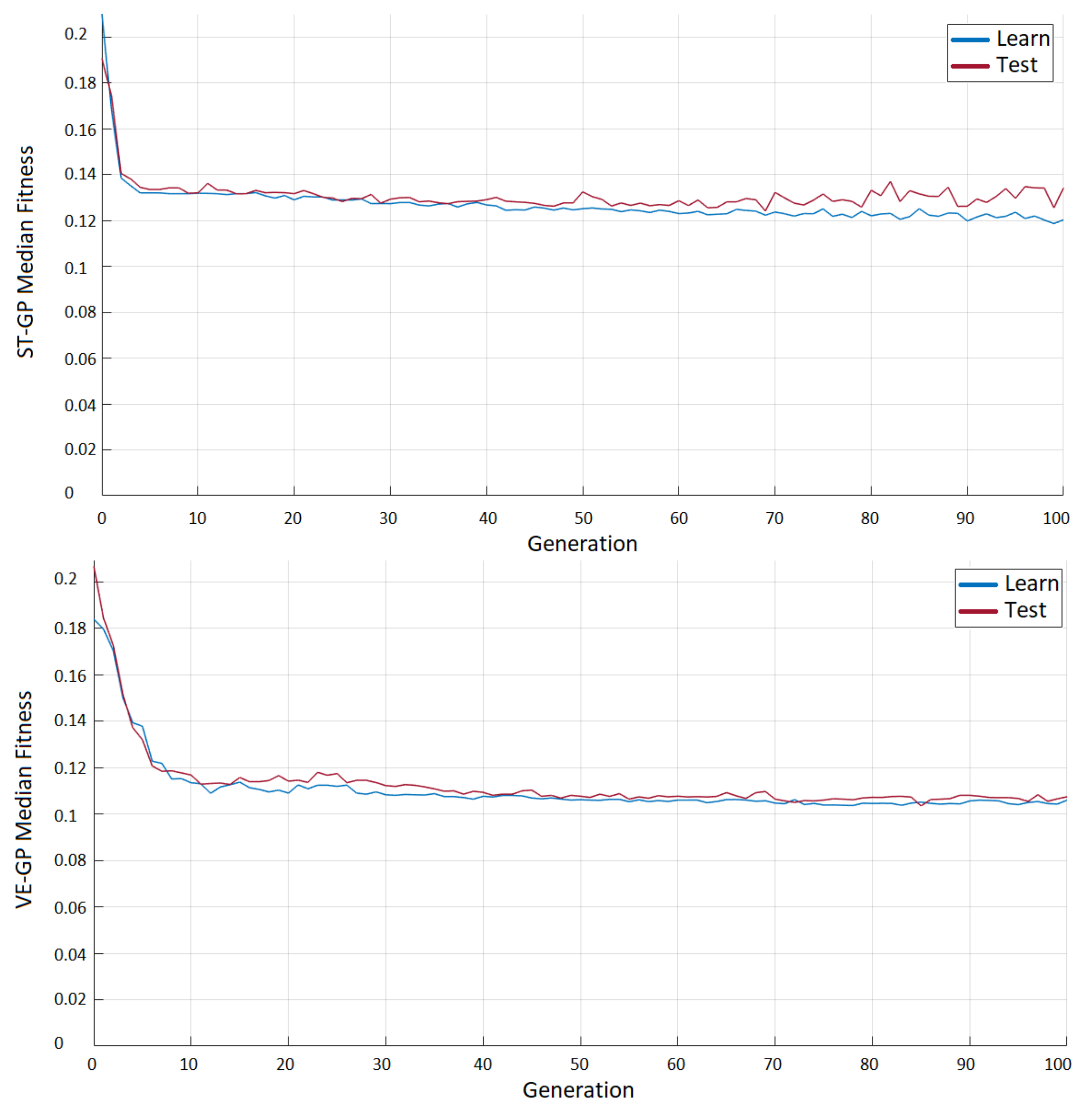
ST-GP and VE-GP were first compared, in order to analyze the behavior of the two algorithms. In Figure 1, the median fitness evolution is plotted, based on the following procedure. For each fold within the learning set, a model was selected according to its performance over the validation set. Hence, after seven runs of the GP, seven models were available, i.e., the ones showing the lowest fitness among the validation. All seven best drawn models were evaluated on the whole learning set and the test set, and the median of the seven models was stored. As the 7-fold was repeated 10 times, 10 median trends were available at the end of the entire evolutionary process. The plot shows the median behavior of the 10 median fitness achieved for each generation. We initially decided to run the two algorithms for 100 generations. The choice of stopping the evolution after 40 generations was dictated by the overfitting trend recorded among ST-GP. On the contrary, VE-GP proved to be more stable than ST-GP, at least as far as we ran 100 generations. Moreover, the median fitness was overall lower, showing that GP is affected by a remarkable improvement of such a problem, if temporal information is added, together with proper functions. The VE-GP models outperformed the ST-GP ones, stabilizing at lower errors. We analyzed the predictors encapsulated in the final models by both ST- and VE-GP, selected with respect to the performance achieved on the test sets by running the algorithms for 40 generations. Table 7 shows that both methods used nine variables to tackle the target. However, the same predictors were not used and, above all, not with the same frequency. The number of , for example, was highly exploited by both GP algorithms, but all the VE-GP models based the prediction on this feature, whereas only 70% of the ST-GP models found it to be informative. , on the other hand, was used only by the ST-GP and in 50% of the solutions, and was involved in 60% of them. was rather exploited only by the VE-GP and in 80% of the models. It is evident that as long as GP is run to predict the target based on the information of a single year, patterns are more difficult to be found, and the algorithm (ST-GP) tries to solve the problem by extracting as much information as possible from as many features as possible (7 variables out of 18 were used in more than 20% and at most in 70% of the solutions). When providing temporal information, the search was easier for GP, whose models achieved better fitness, detecting mainly the information based on a few predictors (4 out of 18 were exploited in more than the 30% of solutions, and among the four features, 1 was handled by all the models). Even considering the variables used by each model (Table 8), on average, 8.4 predictors were used by the ST-GP (from 6 to 15), whereas the VE-GP built models exploiting 5.5 features on average (from 3 to 9).
3.2. Comparisons of ST-GP and VE-GP with Other ML Methods
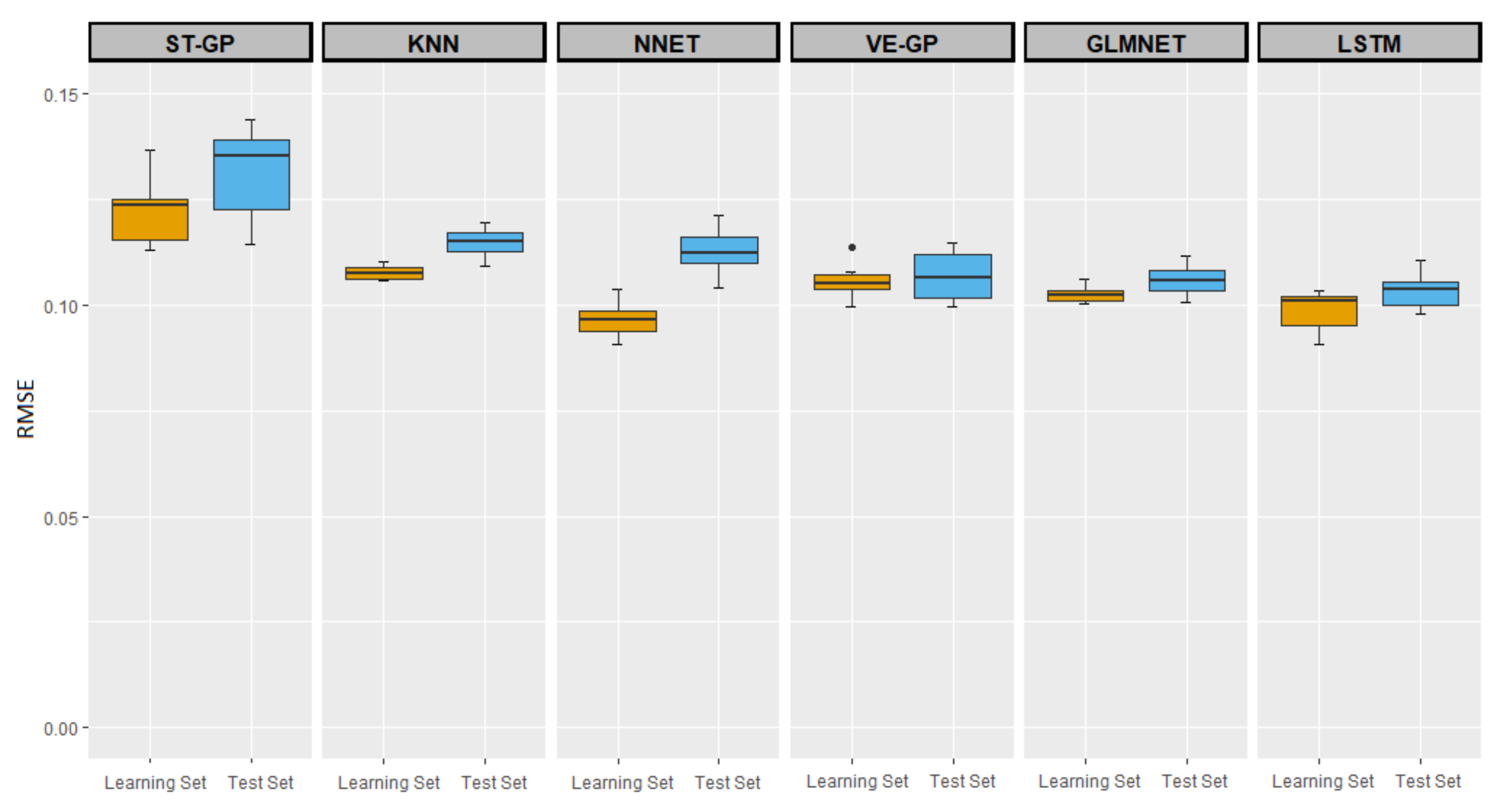
Now, we discuss the results of the experimental comparison between the ST-GP, VE-GP, and the other ML methods presented previously. As already explained, in addition to ST-GP, KNN, NN, and GLMNET also exploited the information on 2017 with a target in 2018, whereas LSTM was involved in the VE-GP to process vectorial variables for 2014–2017 and the 2018 target. The results reported in Section 3.1 for the ST-GP compared to the VE-GP are also supported by the corresponding boxplots in Figure 2. The median and mean RMSE values are reported in Table 9.
The Kruskal–Wallis nonparametric test, performed for all the considered methods with a significance level of = 0.05, was applied to investigate the RMSE achieved among the learning sets and the test sets separately. The resulting p-values (t ≪ 0.001) showed extremely significant differences in median performance between the methods, considering both stages. The pairwise Wilcoxon tests provided with Bonferroni correction = 0.05/15 = 0.0033 was hence performed among all compared techniques. Among the learning set, STGP was significantly different from all other methods, resulting in a poor performance. Likewise, KNN was significantly different with respect to both NN and LSTM, as well as the comparison between VEGP and LSTM. Concerning the RMSE achieved on the test sets, STGP performed poorly with respect to other methods, showing greater, significantly different values for the RMSE on average. On the contrary, GLMNET’s performance was significantly better than KNN’s and NN’s, as well as LSTM’s compared to KNN and VEGP, respectively. Consequently, the following pairs of methods did not show significantly different performance: VEGP–KNN, VEGP–NN, VEGP–GLMNET, VEGP–LSTM, as well as the pair LSTM and GLMNET.
As a further study, we also compared learning and test fitness distributions obtained by the single methods in order to determine the occurrence of overfitting. The Wilcoxon signed rank test showed that the two distributions for KNN and the two obtained with NN were different, since the corresponding p-values were extremely significant (Wilcoxon: p ≪ 0.001), as well as the median RMSE (Kruskal–Wallis test: p ≪ 0.001). Concerning the ST-GP, the two distributions and the median error were slightly different (Wilcoxon and Kruskal–Wallis: p-values equal to 0.048 and 0.034, respectively). GLMNET showed the same learning and test fitness distributions but different median RMSE (Wilcoxon: p > 0.05; Kruskal–Wallis: p = 0.041), whereas LSTM achieved different distributions with similar median. VE-GP was the only method that produced the same fitness distributions with the same median among the learning and test sets.
4. Discussion
Considering all the results of the statistical tests, ST-GP produced less accurate models, and all the other methods outperformed ST-GP. However, among the different techniques, KNN and NN clearly overfitted, generating good results on training data but losing their ability to generalize on unseen data. On the contrary, VE-GP, GLMNET, and LSTM produced better and statistically similar results, as the RMSEs on the test set were not significantly different across these methods. In particular, LSTM produced the best fitness considering both learning and test sets. However, VE-GP was the only method showing the same distribution among learning and test sets, highlighting its ability to generalize better over unseen data. These outcomes are a clear confirmation of the importance of introducing the temporal information in the form of vectors for the studied problem.
The study was dedicated to the inspection of GP behavior when predicting a target starting from datasets that, in one case, were exclusively formed by scalar values (treated hence with ST-GP) and, in the other, assumed a vector representation (handled with VE-GP). This representation is quite useful for incorporating temporal patterns or, in general, successive collections of data for single variables among the same candidate. Indeed, with the common representation through standard data frames, such patterns are usually not recognizable, and the performance of the models do not improve. On the contrary, if the data are organized into a vectorial dataset, the algorithm receives temporal information in input. Thereby, by means of proper functions able to manage vectors, it can produce more accurate predictions. First, the dataset was prepared to deal with the vector-based representation. The datasets, sharing the same scalar target from 2018 (i.e., the quota of weaned calves per cow per year) were prepared by extracting the data among 2017 and among the whole period from 2014–2017, based on a previously defined set of farms. In this study, a different splitting rule was defined among the datasets with respect to previous investigations. The learning and test sets were selected respecting the proportion of 70%–30%, and thereafter, learning sets, randomly reshuffled, were split according to a 7-fold cross validation technique. Prediction models were constructed with different GP algorithms, ST- and VE-GP first, that were thereafter compared with other ML methods. VE-GP was compared with LSTM, which considers the time relationship among the data.
The main goal was hence to inspect the ability of VE-GP with respect to ST-GP in predicting the target. The developed algorithm could produce better results by achieving lower RMSEs among both learning and test sets. We first analyzed the evolution of the median fitness observed on the learning and test sets, and clearly, VE-GP proved to be more stable, evolving a population through more generations without giving sign of overfitting, whereas ST-GP showed the “symptom” quite soon, considering similar experimental settings. In addition, VE-GP reached better results by encapsulating fewer variables in each extracted candidate model, detecting the information to a greater extent from specific features. VE-GP still gave access to the formula and to the features implicitly selected, providing meaningful information about the tackled issue. Being able to extract important features among the predictors in form of vectors, the algorithm improved the target forecast. VE-GP turned out to outperform not only ST-GP but also other techniques used in the field of ML. Although VE-GP performed similarly to LSTM and GLMNET (the latter exploiting the standard data representation), it was the only method that did not show a significantly different behavior on the learning and test sets. The two distributions and their median are similar, entailing that VE-GP provides a good response in terms of generalization ability on unseen data. Improvements can be expected by feeding the algorithm with larger datasets by providing more candidates and longer vectors.
5. Conclusions
Exploring the vectorial approach required, as already stated, a different input data structure. To this purpose, the farms considered in the pool of instances were the same as in [16]. However, since the results showed that GP exploited only certain variables, the number of predictors was reduced to 18. In this way, possible noise due to extra variables, which were not very informative, was avoided. The main goal was to inspect the ability of Vectorial Genetic Programming (VE-GP) with respect to ST-GP to predict the target. The recently developed VE-GP algorithm could produce better results, by achieving a better fitness on both the learning and test sets. VE-GP proved to be more stable, evolving a population through more generations without showing overfitting, while Standard Genetic Programming (ST-GP), was affected by overfitting already in the early generations under analogous experimental settings. VE-GP still favored model investigation by giving access to the formula and hence to the features implicitly selected, providing meaningful information about the tackled issue. Better results were obtained by encapsulating fewer variables in each extracted candidate model, detecting almost all the information among specific features. The algorithm improved the target forecast, proving to outperform not only ST-GP, but also other techniques used in the field of ML. The algorithm, in particular, was compared to Long Short-Term Memory Recurrent Neural Network (LSTM), suitable for handling vectorial predictors. Even though performing similar to the LSTM and Generalized Linear Models (GLMNET), the latter exploiting the standard data panel representation, VE-GP was the only method entailing a greater ability in generalization over unseen data.
The introduction of vectorial variables produced a significant improvement over the accuracy of the result. Evolution was also much more stable, and the ability of the algorithm to handle any type of variable, both scalar and vectorial, makes it quite a flexible tool. These considerations open the possibility of providing more complex datasets, containing different types of sequential features. The possibility of managing vectorial variables, whose values can be of different types and have no fixed length among the whole dataset, push the analysis beyond the basic research conducted at this point. On the one side, both categorical and continuous variables can be treated simultaneously, without specifying it explicitly to the algorithm: The latter is indeed able to process them during the evolution without hints given by the user. On the other hand, when dealing with vectors, some data may be not available. Thus, the vector variables may have different lengths, even being scalars when the latter is equal to one. VE-GP is suitable to manage all kinds of features dynamically, combining them in the prediction of the target. Evolutionary algorithms can be applied to zootechnical data, achieving performing models able to learn from all the available data. In this case study, the breeding variables in the report extracted at the end of the year were used. In one case, they were managed for only one year; in the other four, the average values, corresponding to four years, were used, proving to be more suitable for reducing the prediction and generalization errors. Instead of limiting the analysis to the year-end average, it might be more useful to incorporate the data collected from each farm visit into a vector representation. As a result, all variations, even small ones, would be available, and the algorithm could identify temporal patterns that were not visible by directly processing the average value for the whole year.
Author Contributions
Conceptualization, F.A. and M.G.; methodology, F.A., L.V., and M.G.; validation, L.V. and M.G.; formal analysis, F.A.; investigation, F.A.; resources, F.A.; data curation, F.A.; writing—original draft preparation, F.A.; writing—review and editing, F.A. and M.G.; visualization, F.A.; supervision, L.V. and M.G.; project administration, M.G. All authors have read and agreed to the published version of the manuscript.
Funding
This work was partially supported by FCT, Portugal, through funding of projects BINDER (PTDC/CCI-INF/29168/2017) and AICE (DSAIPA/DS/0113/2019).
Conflicts of Interest
The authors declare no conflict of interest.
Abbreviations
The following abbreviations are used in this manuscript:
| PLF | Precision Livestock Farming |
| ML | Machine Learning |
| ANABORAPI | National Association of Piemontese Cattle Breeders |
| GP | Genetic Programming |
| ST-GP | Standard Genetic Programming |
| VE-GP | Vectorial Genetic Programming |
| EA | Evolutionary Algorithm |
| KNN | k-Nearest Neighbors |
| NN | Neural Network |
| LM | Linear Model |
| GLMNET | Generalized Linear Model with Elastic Net Regularization |
| RNN | Recurrent Neural Network |
| LSTM | Long Short-Term Memory |
References
- Berckmans, D. Precision livestock farming technologies for welfare management in intensive livestock systems. Rev. Sci. Tech. 2014, 33, 189–196. [Google Scholar] [CrossRef] [PubMed]
- Berckmans, D.; Guarino, M. Precision livestock farming for the global livestock sector. Anim. Front. 2017, 7, 4–5. [Google Scholar] [CrossRef] [Green Version]
- Cole, J.B.; Newman, S.; Foertter, F.; Aguilar, I.; Coffey, M. Breeding and Genetics Symposium: Really big data: Processing and analysis of very large datasets. J. Anim. Sci. 2012, 90, 723–733. [Google Scholar] [CrossRef] [PubMed]
- Lokhorst, C.; de Mol, R.M.; Kamphuis, C. Invited review: Big Data in precision dairy farming. Animal 2012, 13, 1519–1528. [Google Scholar] [CrossRef] [PubMed] [Green Version]
- Berckmans, D. General introduction to precision livestock farming. Anim. Front. 2017, 7, 6–11. [Google Scholar] [CrossRef]
- Halachmi, I.; Guarino, M. Editorial: Precision livestock farming: A ’per animal’ approach using advanced monitoring technologies. Anim. Int. J. Anim. Biosci. 2016, 10, 1482–1483. [Google Scholar] [CrossRef] [PubMed] [Green Version]
- Liakos, K.; Busato, P.; Moshou, D.; Pearson, S.; Bochtis, D. Machine Learning in Agriculture: A Review. Sensors 2018, 18, 2674. [Google Scholar] [CrossRef] [PubMed] [Green Version]
- Morota, G.; Ventura, R.V.; Silva, F.F.; Koyama, M.; Fernando, S.C. Big data analytics and precision animal agriculture symposium: Machine learning and data mining advance predictive big data analysis in precision animal agriculture. J. Anim. Sci. 2018, 96, 1540–1550. [Google Scholar] [CrossRef] [PubMed]
- Gahegan, M. Is inductive machine learning just another wild goose (or might it lay the golden egg)? Int. J. Geogr. Inf. Sci. 2003, 17, 69–92. [Google Scholar] [CrossRef]
- Craninx, M.; Fievez, V.; Vlaeminck, B.; Baets, B. Artificial neural network models of the rumen fermentation pattern in dairy cattle. Comput. Electron. Agric. 2008, 60, 226–238. [Google Scholar] [CrossRef]
- Gonzalez-Recio, O.; Rosa, G.J.M.; Gianola, D. Machine learning methods and predictive ability metrics for genome-wide prediction of complex traits. Livest. Sci. 2014, 166, 217–231. [Google Scholar] [CrossRef]
- Yao, C.; Zhu, X.; Weigel, K.A. Semi-supervised learning for genomic prediction of novel traits with small reference populations: An application to residual feed intake in dairy cattle. Genet. Sel. Evol. 2016, 48, 84. [Google Scholar] [CrossRef] [PubMed] [Green Version]
- Associazione Nazionale Allevatori Bovini Razza Piemontese. Available online: http://www.anaborapi.it (accessed on 8 December 2021).
- Bona, M.; Albera, A.; Bittante, G.; Moretta, A.; Franco, G. L’allevamento della manza e della vacca piemontese. Tec. Allev. 2005, 44, 65–129. [Google Scholar]
- Abbona, F.; Vanneschi, L.; Bona, M.; Giacobini, M. A GP approach for precision farming. In Proceedings of the 2020 IEEE Congress on Evolutionary Computation (CEC), Glasgow, UK, 19–24 July 2020; pp. 1–8. [Google Scholar]
- Abbona, F.; Vanneschi, L.; Bona, M.; Giacobini, M. Towards modelling beef cattle management with Genetic Programming. Livest. Sci. 2020, 241, 104205. [Google Scholar] [CrossRef]
- Abraham, A.; Nedjah, N.; Mourelle, L.M. Evolutionary Computation: From Genetic Algorithms to Genetic Programming. In Genetic Systems Programming; Springer: Berlin/Heidelberg, Germany, 2006. [Google Scholar]
- Azzali, I.; Vanneschi, L.; Silva, S.; Bakurov, I.; Giacobini, M. A Vectorial Approach to Genetic Programming. In Proceedings of the EuroGP 2019, Leipzig, Germany, 24–26 April 2019. [Google Scholar]
- Azzali, I.; Vanneschi, L.; Bakurov, I.; Silva, S.; Ivaldi, M.; Giacobini, M. Towards the use of vector based GP to predict physiological time series. Appl. Soft Comput. 2020, 89, 106097. [Google Scholar] [CrossRef] [Green Version]
- Koza, J. Genetic programming as a means for programming computers by natural selection. Stat. Comput. 1994, 4, 87–112. [Google Scholar] [CrossRef]
- Poli, R.; Langdon, W.; McPhee, N. A Field Guide to Genetic Programming; Lulu Enterprises, UK Ltd.: Egham, UK, 2008. [Google Scholar]
- Spiess, A.; Neumeyer, N. An evaluation of R2 as an inadequate measure for nonlinear models in pharmacological and biochemical research: A Monte Carlo approach. BMC Pharmacol. 2010, 10, 6. [Google Scholar] [CrossRef] [PubMed] [Green Version]
- Alfaro-Cid, E.; Sharman, K.; Esparcia-Alcázar, A. Genetic Programming and Serial Processing for Time Series Classification. Evol. Comput. 2014, 22, 265–285. [Google Scholar] [CrossRef]
- Bartashevich, P.; Bakurov, I.; Mostaghim, S.; Vanneschi, L. A Evolving PSO algorithm design in vector fields using geometric semantic GP. In Proceedings of the Genetic and Evolutionary Computation Conference Companion, Kyoto, Japan, 15–19 July 2018. [Google Scholar]
- Holladay, K.; Robbins, K.A. Evolution of Signal Processing Algorithms using Vector Based Genetic Programming. In Proceedings of the 2007 15th International Conference on Digital Signal Processing, Cardiff, UK, 1–4 July 2007; pp. 503–506. [Google Scholar]
- Silva, S. GPLAB—A Genetic Programming Toolbox for MATLAB. 2007. Available online: http://gplab.sourceforge.net/index.html (accessed on 8 December 2021).
- Kuhn, M. Classification and Regression Training [R Package Caret Version 6.0-86]. 2020. Available online: https://cran.r-project.org/web/packages/caret/caret.pdf (accessed on 8 December 2021).
- Lantz, B. Machine Learning with R, 2nd ed.; Packt Publishing: Birmingham, UK; Cambridge University Press: Cambridge, UK, 2015. [Google Scholar]
Figure 1.
ST-GP (up) and VE-GP (down) fitness evolution plots. For each generation, the graph plots the median of the 10 median fitness achieved by the best 7 models on the validation sets and correspondingly the performance achieved on the learning and test sets.
Figure 1.
ST-GP (up) and VE-GP (down) fitness evolution plots. For each generation, the graph plots the median of the 10 median fitness achieved by the best 7 models on the validation sets and correspondingly the performance achieved on the learning and test sets.

Figure 2.
RMSEs on both the learning and test sets for the different algorithms. Learning results are plotted in yellow (left) and test results are plotted in blue (right) for each technique.
Figure 2.
RMSEs on both the learning and test sets for the different algorithms. Learning results are plotted in yellow (left) and test results are plotted in blue (right) for each technique.


Table 1.
Standard Data Panel. Structure of the dataset. The farms are listed horizontally, as well as the reference year, the variables vertically.
Table 1.
Standard Data Panel. Structure of the dataset. The farms are listed horizontally, as well as the reference year, the variables vertically.
| FARM | YEAR | PRIMIPAROUS | PLURIPAROUS | HEIFERS | INTERPARTO |
|---|---|---|---|---|---|
| Farm 1 | 2014 | 22 | 36 | 7 | 365 |
| Farm 1 | 2015 | 10 | 46 | 13 | 375 |
| Farm 1 | 2016 | 16 | 47 | 12 | 381 |
| Farm 1 | 2017 | 14 | 46 | 11 | 375 |
| Farm 1 | 2018 | 16 | 47 | 12 | 374 |
| Farm 2 | 2014 | 11 | 90 | 9 | 396 |
| Farm 2 | 2015 | 10 | 93 | 9 | 391 |
| Farm 2 | 2016 | 9 | 95 | 7 | 380 |
| Farm 2 | 2017 | 7 | 97 | 10 | 387 |
| Farm 2 | 2018 | 9 | 92 | 11 | 385 |
| Farm 3 | 2014 | 7 | 42 | 3 | 414 |
| Farm 3 | 2015 | 4 | 43 | 4 | 439 |
| Farm 3 | 2016 | 4 | 44 | 10 | 452 |
| Farm 3 | 2017 | 10 | 44 | 11 | 425 |
| Farm 3 | 2018 | 9 | 60 | 4 | 473 |
Table 2.
Final set of variables used for the benchmarked problem. The bottom line represents the dependent variable Y, i.e., the target for the predicted models.
Table 2.
Final set of variables used for the benchmarked problem. The bottom line represents the dependent variable Y, i.e., the target for the predicted models.
| Variable Name | Variable Description | |
|---|---|---|
| 1 | Consistency for cows, i.e., number of cows | |
| 2 | Consistency for heifers, i.e., number of heifers | |
| 3 | Calving interval in days, based on currently pregnant cows | |
| 4 | Average parity | |
| 5 | __1 | Age at first calving |
| 6 | N. of cows that delivered with easy calving | |
| 7 | N. of primiparous that delivered with easy calving | |
| 8 | _ | Calving ease (EBV for cows) |
| 9 | _ | Birth ease (EBV for heifers) |
| 10 | Birth ease (EBV for A.I. bulls) | |
| 11 | Calving ease (EBV for A.I. bulls) | |
| 12 | UBA referred to bovines 6 months–2 years old | |
| 13 | UBA referred to bovines 4–6 months old | |
| 14 | N. of dead calves in the first 60 days after birth | |
| 15 | Total number of calves born | |
| 16 | Total number of calves born alive | |
| 17 | Percentage of calves born without defects (e.g., Macroglossia, Arthrogryposis) | |
| 18 | _ | Consanguinity calculated on future calves |
| 19 | Y | N. of weaned calves per cow per year (2) |
Table 3.
Dataset configuration from 2017–2018. On the left side, the input scalar variables . On the right side, the scalar target .
Table 3.
Dataset configuration from 2017–2018. On the left side, the input scalar variables . On the right side, the scalar target .
| 2017 | 2018 | ||||||
|---|---|---|---|---|---|---|---|
COWS | COW_AGE | CALVING_INT | N_CALVING | ||||
| FARM 1- | 104 | 3020 | 387 | 60 | 0.95 | ||
| FARM 2- | 54 | 3112 | 425 | 54 | 0.9 | ||
| FARM 3- | 63 | 2824 | 515 | 48 | 0.69 | ||
| … | 49 | 3131 | 466 | 49 | 0.67 | ||
| 108 | 2766 | 407 | 50 | 0.85 | |||
| 74 | 3448 | 459 | 62 | 0.84 | |||
Table 4.
Vectorial panel dataset configuration for 2014–2018. On the left side, the input vectorial variables , with , , and . On the right side, the scalar target variable .
Table 4.
Vectorial panel dataset configuration for 2014–2018. On the left side, the input vectorial variables , with , , and . On the right side, the scalar target variable .
| 2014–2017 | 2018 | |||||
|---|---|---|---|---|---|---|
COWS | COW_AGE | CALVING_INT | ||||
| FARM 1- | [98, 101, 107, 104] | [2999, 3001, 2998, 3020] | [391, 391, 380, 387] | 0.95 | ||
| FARM 2- | [61, 49, 53, 54] | [3076, 3002, 3056, 3112] | [408, 376, 402, 425] | 0.9 | ||
| FARM 3- | [53, 55, 64, 63] | [2799, 2813, 2802, 2824] | [367, 376, 406, 515] | 0.69 | ||
| … | [31, 36, 47, 49] | [3102, 3075, 3009, 3131] | [434, 480, 461, 466] | 0.67 | ||
| [102, 99, 105, 108] | [2704, 2795, 2789, 2766] | [404, 371, 395, 407] | 0.85 | |||
| [69, 71, 75, 74] | [3401, 3388, 3406, 3448] | [387, 367, 373, 459] | 0.84 | |||
Table 5.
Parameters used to perform GP.
| Parameter | Description |
|---|---|
| ST-GP | |
| Maximum number of generations | 40 |
| Population size | 250 |
| Selection Method | Lexicographic Parsimony Pressure |
| Elitism | Keepbest |
| Initialization Method | Ramped half and half |
| Tournament Size | 2 |
| Subtree Crossover Rate | 0.7 |
| Subtree Mutation Rate | 0.1 |
| Subtree Shrinkmutation Rate | 0.1 |
| Subtree Swapmutation Rate | 0.1 |
| Maxtreedepth | 17 |
| VE-GP | |
| Maximum number of generations | 40 |
| Population size | 250 |
| Selection Method | Lexicographic Parsimony Pressure |
| Elitism | Keepbest |
| Initialization Method | Ramped half and half |
| Tournament Size | 2 |
| Subtree Crossover Rate | 0.7 |
| Subtree Mutation Rate | 0.3 |
| Mutation of aggregate function parameters | 0.2 |
| Maxtreedepth | 17 |
Table 6.
Parameters used to perform ML techniques with caret package in R and the Deep Learning Toolbox in MATLAB.
Table 6.
Parameters used to perform ML techniques with caret package in R and the Deep Learning Toolbox in MATLAB.
| ML Technique | Parameters |
|---|---|
| knn | k = 15 |
| nnet | size = 7; decay = 0.2 |
| glmnet | = 0.8, = 0.85 |
| LSTM | hidden units = 200; epochs = 50; batchsize = 1; learning algorithm = adam. |
Table 7.
Frequency of use of each variable among the best 10 individuals found by ST-GP (left column) and VE-GP (right column).
Table 7.
Frequency of use of each variable among the best 10 individuals found by ST-GP (left column) and VE-GP (right column).
| Variable | % of Use (ST-GP) | % of Use (VE-GP) |
|---|---|---|
| X1 | 70% | 100% |
| X2 | 10% | 10% |
| X3 | 0% | 10% |
| X4 | 50% | 0% |
| X5 __1 | 0% | 10% |
| X6 | 0% | 10% |
| X7 | 0% | 10% |
| X8 _ | 0% | 0% |
| X9 _ | 0% | 0% |
| X10 | 10% | 0% |
| X11 | 0% | 0% |
| X12 | 0% | 0% |
| X13 | 20% | 0% |
| X14 | 70% | 40% |
| X15 | 0% | 80% |
| X16 | 60% | 0% |
| X17 | 30% | 0% |
| X18 _ | 20% | 30% |
Table 8.
Fitness on the test set, number of involved variables, and corresponding percentage for each model evolved by ST-GP (upper table) and VE-GP (lower table) in each of the 10 runs.
Table 8.
Fitness on the test set, number of involved variables, and corresponding percentage for each model evolved by ST-GP (upper table) and VE-GP (lower table) in each of the 10 runs.
| Prediction Model | Fitness on Test | N. of Variables | % of Variables |
|---|---|---|---|
| ST-GP | |||
| model 1 | 0.1335 | 9 | 50% |
| model 2 | 0.1207 | 6 | 33% |
| model 3 | 0.1143 | 11 | 61% |
| model 4 | 0.1383 | 8 | 44% |
| model 5 | 0.1392 | 7 | 39% |
| model 6 | 0.1439 | 7 | 39% |
| model 7 | 0.1395 | 8 | 44% |
| model 8 | 0.1370 | 6 | 33% |
| model 9 | 0.1285 | 15 | 83% |
| model 10 | 0.1184 | 7 | 39% |
| VE-GP | |||
| model 1 | 0.1117 | 5 | 26% |
| model 2 | 0.1016 | 3 | 16% |
| model 3 | 0.1044 | 9 | 47% |
| model 4 | 0.1085 | 8 | 42% |
| model 5 | 0.1134 | 3 | 16% |
| model 6 | 0.0998 | 8 | 42% |
| model 7 | 0.1018 | 4 | 21% |
| model 8 | 0.1149 | 4 | 21% |
| model 9 | 0.0999 | 8 | 42% |
| model 10 | 0.1121 | 3 | 16% |
Table 9.
Median and mean RMSE of the different techniques among the learning and test sets.
| STGP | KNN | NN | VEGP | GLMNET | LSTM | |
|---|---|---|---|---|---|---|
| Learning sets | ||||||
| Median | 0.1238 | 0.1074 | 0.0967 | 0.1052 | 0.1025 | 0.1011 |
| Mean | 0.1220 | 0.1077 | 0.0967 | 0.1054 | 0.1025 | 0.0988 |
| Test sets | ||||||
| Median | 0.1353 | 0.1151 | 0.1122 | 0.1065 | 0.1057 | 0.1037 |
| Mean | 0.1314 | 0.1147 | 0.1128 | 0.1068 | 0.1056 | 0.1034 |
Publisher’s Note: MDPI stays neutral with regard to jurisdictional claims in published maps and institutional affiliations. |
© 2022 by the authors. Licensee MDPI, Basel, Switzerland. This article is an open access article distributed under the terms and conditions of the Creative Commons Attribution (CC BY) license (https://creativecommons.org/licenses/by/4.0/).
Share and Cite
MDPI and ACS Style
Abbona, F.; Vanneschi, L.; Giacobini, M. Towards a Vectorial Approach to Predict Beef Farm Performance. Appl. Sci. 2022, 12, 1137. https://doi.org/10.3390/app12031137
AMA Style
Abbona F, Vanneschi L, Giacobini M. Towards a Vectorial Approach to Predict Beef Farm Performance. Applied Sciences. 2022; 12(3):1137. https://doi.org/10.3390/app12031137
Chicago/Turabian StyleAbbona, Francesca, Leonardo Vanneschi, and Mario Giacobini. 2022. "Towards a Vectorial Approach to Predict Beef Farm Performance" Applied Sciences 12, no. 3: 1137. https://doi.org/10.3390/app12031137
Note that from the first issue of 2016, this journal uses article numbers instead of page numbers. See further details here.