
Estimation of Water Coverage in Permanent and Temporary Shallow Lakes and Wetlands by Combining Remote Sensing Techniques and Genetic Programming: Application to the Mediterranean Basin of the Iberian Peninsula

 ,
,  , , and
Abstract
:
1. Introduction
2. Materials and Methods
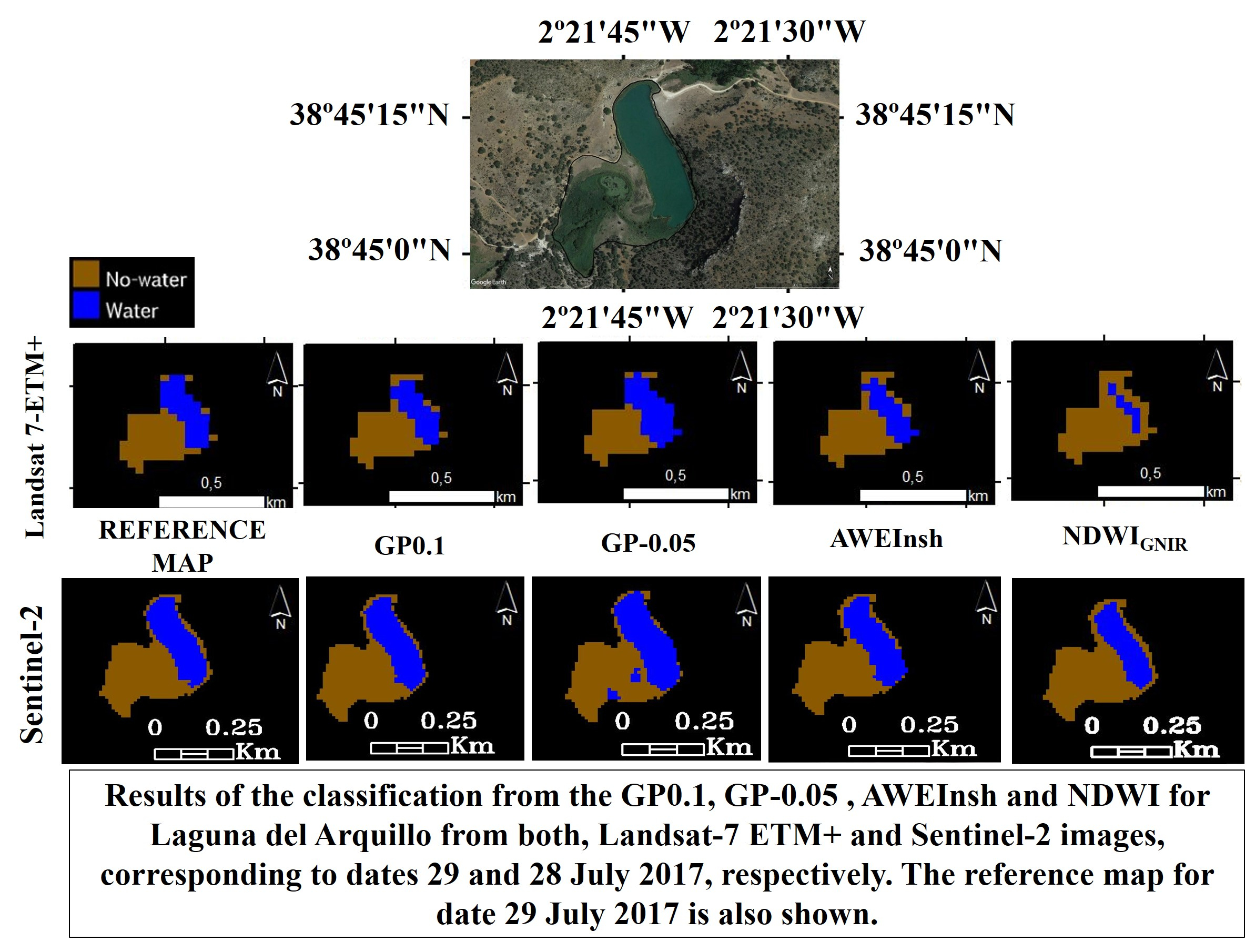
2.1. Study Area
2.2. Reference Data
2.3. Remote Sensing Data Collection and Pre-Processing
2.4. Water Mapping Method
3. Results
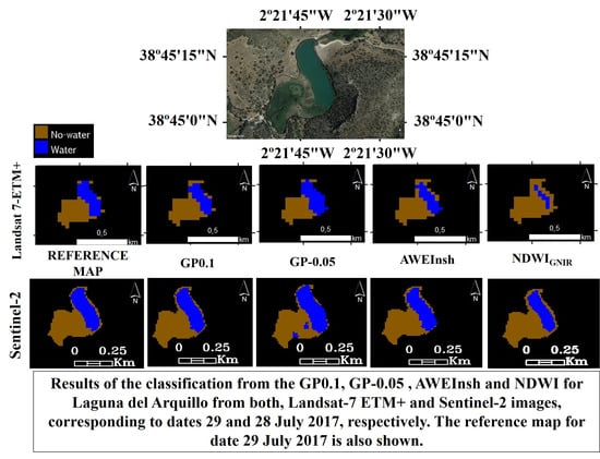
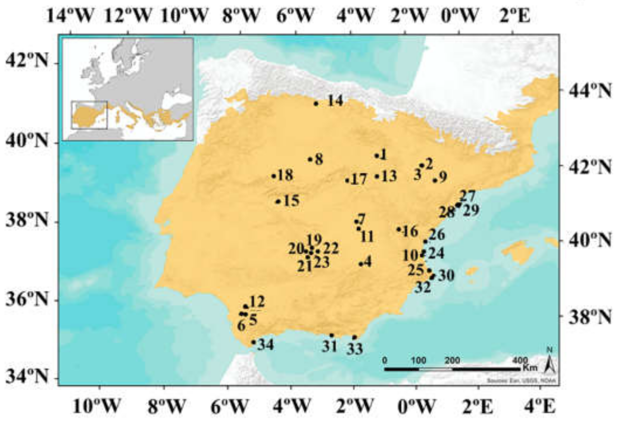
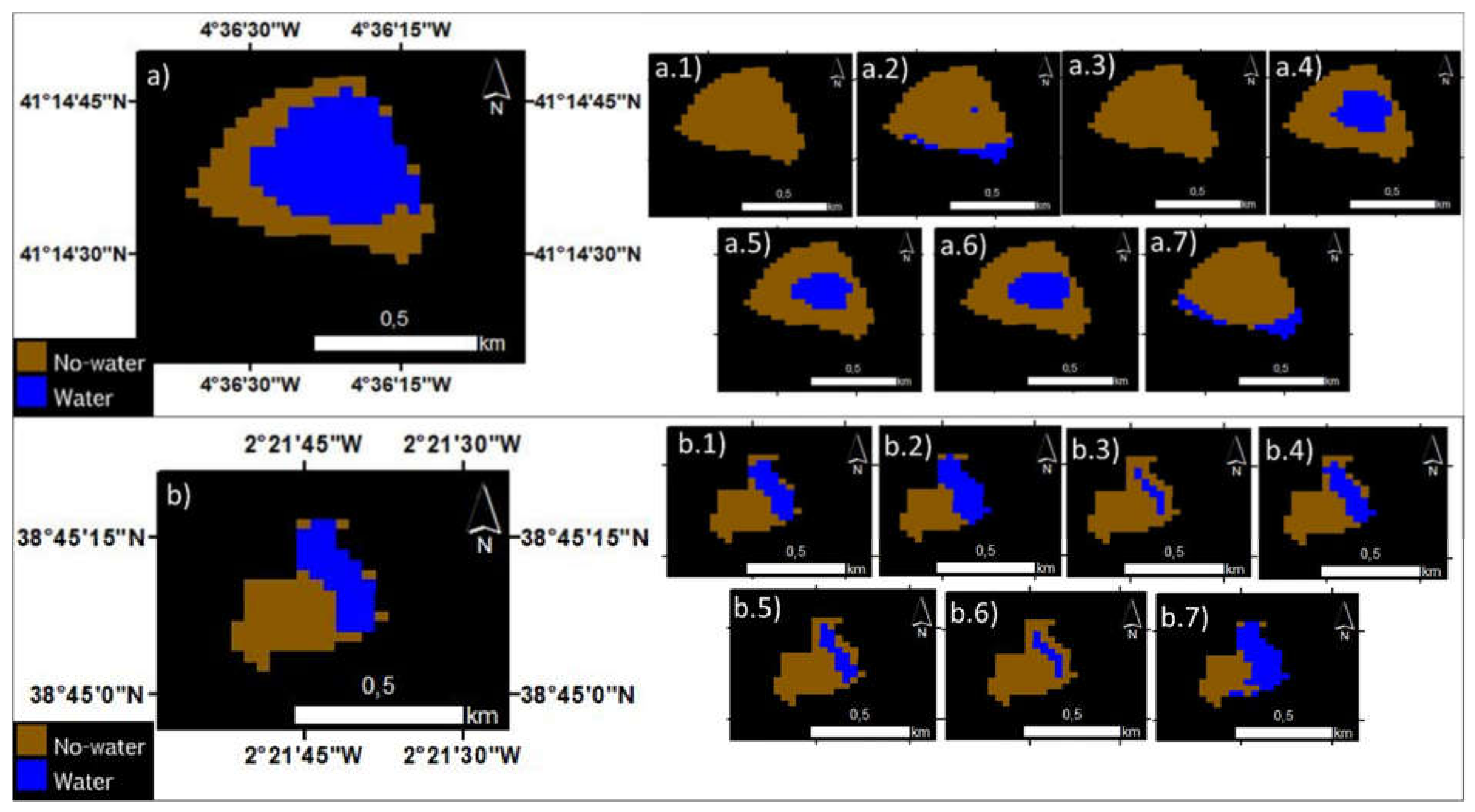
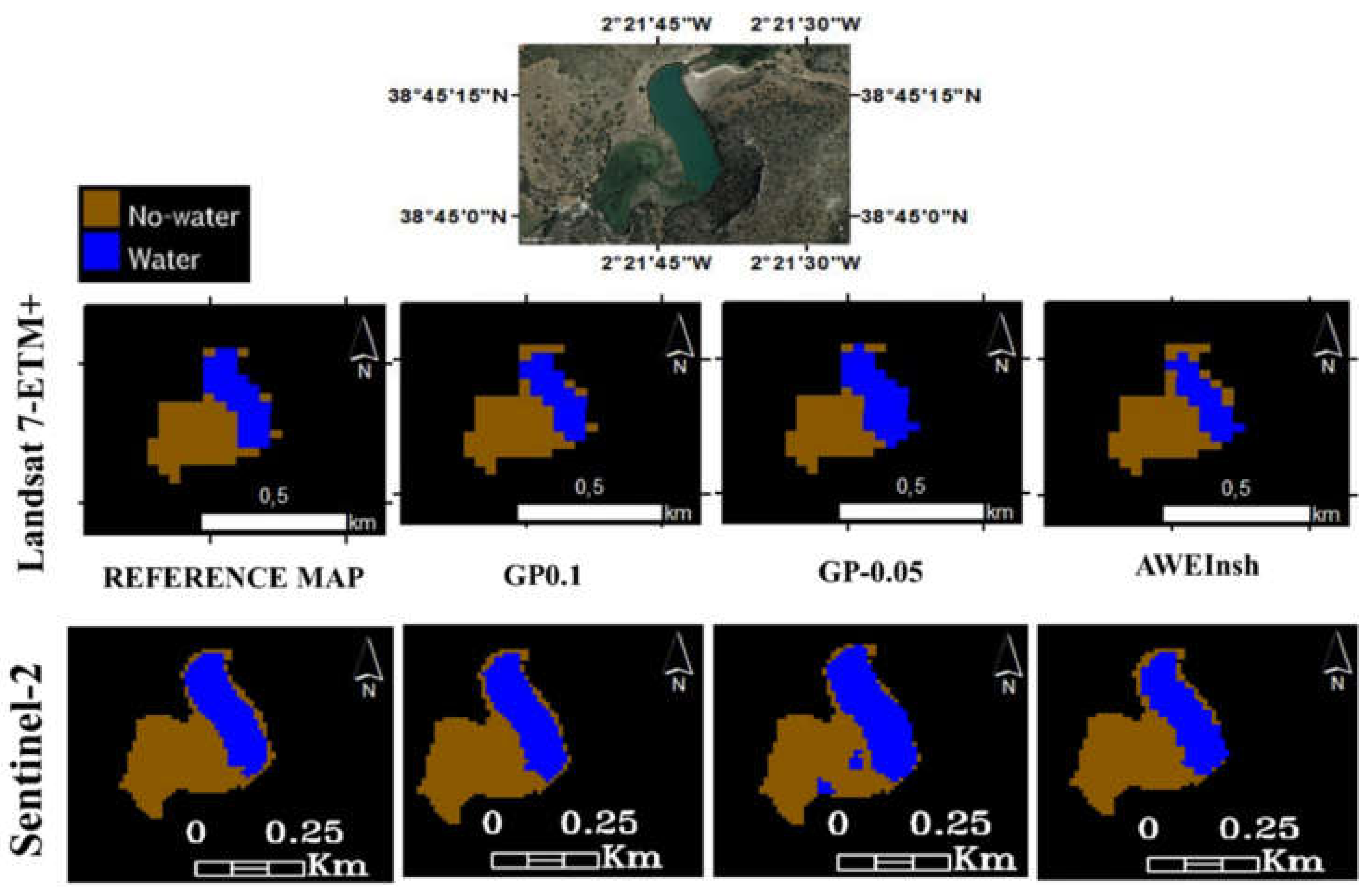
3.1. Landsat-7 ETM+ Imagery
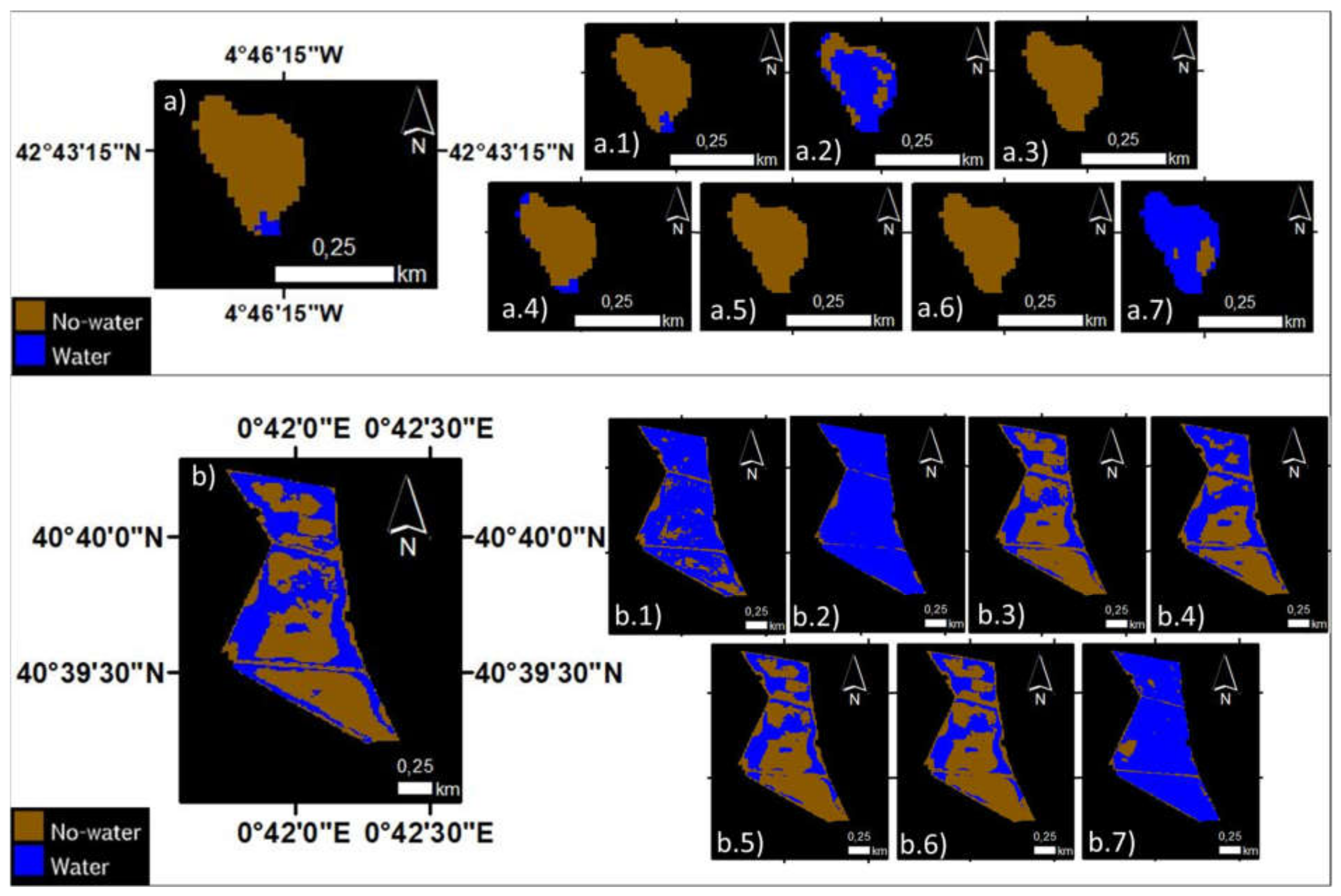
3.2. Sentinel-2 Imagery
4. Discussion
5. Conclusions
Supplementary Materials
Author Contributions
Funding
Institutional Review Board Statement
Informed Consent Statement
Data Availability Statement
Conflicts of Interest
References
- Vives, P.T. Monitoring Mediterranean Wetlands: A Methodological Guide; MedWet, Wetlands International: Slimbridge, UK; ICN: Lisbon, Portugal, 1996; ISBN 1-900442-04-3. [Google Scholar]
- Camacho, A.; Peinado, R.; Santamans, A.C.; Picazo, A. Functional ecological patterns and the effect of anthropogenic disturbances on a recently restored Mediterranean coastal lagoon: Needs for a sustainable restoration. Estuar. Coast. Shelf Sci. 2012, 114, 105–117. [Google Scholar] [CrossRef]
- Gardner, R.C.; Barchiesi, S.; Beltrame, C.; Finlayson, C.M.; Galewski, T.; Harrison, I.; Paganini, M.; Perennou, C.; Pritchard, D.; Rosenqvist, A.; et al. State of the world’s wetlands and their services to people: A compilation of recent analyses. In Ramsar Briefing Note No.7; Ramsar Convention Secretariat: Gland, Switzerland, 2015. [Google Scholar]
- Ramsar Convention Secretariat. Regional overview of the implementation of the convention and its strategic plan in Europe. In Proceedings of the Report to the 12th Meeting of the Conference of the Parties to the Convention on Wetlands, Punta del Este, Uruguay, 2–9 June 2015; pp. 1–9. [Google Scholar]
- Perennou, C.; Guelmami, A.; Paganini, M.; Philipson, P.; Poulin, B.; Strauch, A.; Tottrup, C.; Truckenbrodt, J.; Geijzendorffer, I.R. Chapter Six—Mapping Mediterranean Wetlands With Remote Sensing: A Good-Looking Map Is Not Always a Good Map. Adv. Ecol. Res. 2018, 58, 243–277. [Google Scholar]
- Castañeda, C.; Herrero, J. Teledetección de Cambios en la Laguna de Gallocanta. Mem. R. Soc. Esp. Hist. Nat. 2009, 7, 103–126. [Google Scholar]
- Bai, J.; Chen, X.; Li, J.; Yang, L.; Fang, H. Changes in the Area of Inland Lakes in Arid Regions of Central Asia during the past 30 years. Environ. Monit. Assess. 2011, 178, 247–256. [Google Scholar] [CrossRef]
- McFeeters, S.K. Using the Normalized Difference Water Index (NDWI) within a Geographic Information System to detect Swimming Pools for Mosquito Abatement: A Practical Approach. Remote Sens. 2013, 5, 3544–3561. [Google Scholar] [CrossRef] [Green Version]
- Ji, L.; Zhang, L.; Wylie, B. Analysis of Dynamic Thresholds for the Normalized Difference Water Index. Photogramm. Eng. Remote Sens. 2009, 75, 1307–1317. [Google Scholar] [CrossRef]
- Klein, I.; Dietz, A.J.; Gessner, U.; Galayeva, A.; Myrzakhmetov, A.; Kuenzer, C. Evaluation of Seasonal Water Body Extents in Central Asia over the past 27 years derived from Medium-Resolution Remote Sensing Data. Int. J. Appl. Earth Obs. Geoinf. 2014, 26, 335–349. [Google Scholar] [CrossRef]
- Moser, L.; Voigt, S.; Schoepfer, E. Monitoring of critical water and vegetation anomalies of Sub-Saharan West-African Wetlands. In Proceedings of the 2014 IEEE Geoscience and Remote Sensing Symposium (IGARSS), Quebec City, QC, Canada, 13–18 July 2014; pp. 3842–3845. [Google Scholar]
- Lefebvre, G.; Willm, L.; Campagna, J.; Redmond, L. Introducing WIW for Detecting the Presence of Water in Wetlands with Landsat and Sentinel Satellites. Remote Sens. 2019, 11, 2210. [Google Scholar] [CrossRef] [Green Version]
- Campos, J.C.; Sillero, N.; Brito, J.C. Normalized Difference Water Indexes have Dissimilar Performances in detecting Seasonal and Permanent Water in the Sahara-Sahel Transition Zone. J. Hydrol. 2012, 464–465, 438–446. [Google Scholar] [CrossRef]
- Doña, C.; Sanchez, J.M.; Caselles, V.; Dominguez, J.A.; Camacho, A. Empirical Relationships for Monitoring Water Quality of Lakes and Reservoirs Through Multispectral Images. IEEE J. Sel. Top. Appl. Earth Obs. Remote Sens. 2014, 7, 1632–1641. [Google Scholar] [CrossRef]
- Doña, C.; Chang, N.B.; Caselles, V.; Sánchez, J.M.; Camacho, A.; Delegido, J.; Vannah, B.W. Integrated Satellite Data Fusion and Mining for Monitoring Lake Water Quality Status of the Albufera de Valencia in Spain. J. Environ. Manag. 2015, 151, 416–426. [Google Scholar] [CrossRef] [Green Version]
- Copernicus Global Land Service Site. Available online: https://land.copernicus.eu/global/ (accessed on 26 December 2020).
- Kaplan, G.; Avdan, U. Mapping and monitoring wetlands using sentinel-2 satellite imagery. In Proceedings of the 4th International GeoAdvances Workshop, Karabuk, Turkey, 14–15 October 2017; Volume IV-4/W4, pp. 271–277. [Google Scholar]
- Araya-lópez, R.A.; Lopatin, J.; Fassnacht, F.E.; Hernández, H.J. Monitoring Andean High Altitude Wetlands in Central Chile with Seasonal Optical Data: A Comparison between Worldview-2 and Sentinel-2 imagery. ISPRS J. Photogramm. Remote Sens. 2018, 145, 213–224. [Google Scholar] [CrossRef]
- Bustamante, J.; Díaz-Delgado, R.; Aragonés, D. Determinación de las Características de Masas de Aguas Someras en las Marismas de Doñana mediante Teledetección. Rev. Teledetec. 2005, 24, 107–111. [Google Scholar]
- Doña, C.; Chang, N.B.; Caselles, V.; Sánchez, J.M.; Pérez-Planells, L.; Bisquert, M.; García-Santos, V.; Imen, S. Monitoring Hydrological Patterns of Temporary Lakes Using Remote Sensing and Machine Learning Models: Case Study of La Mancha Húmeda Biosphere Reserve in Central Spain. Remote Sens. 2016, 8, 618. [Google Scholar] [CrossRef] [Green Version]
- Jain, S.K.; Singh, R.D.; Jain, M.K.; Lohani, A.K. Delineation of Flood-Prone Areas using Remote Sensing Techniques. Water Resour. Manag. 2005, 19, 333–347. [Google Scholar] [CrossRef]
- Ouma, Y.O.; Tateishi, R. A water index for rapid mapping of shoreline changes of five East African Rift Valley lakes: An empirical analysis using Landsat TM and ETM+ data. Int. J. Remote Sens. 2006, 27, 3153–3181. [Google Scholar] [CrossRef]
- Lira, J. Segmentation and Morphology of Open Water Bodies from Multispectral Images. Int. J. Remote Sens. 2006, 27, 4015–4038. [Google Scholar] [CrossRef]
- Fisher, A.; Danaher, T. A Water Index for SPOT5 HRG Satellite Imagery, New South Wales, Australia, Determined by Linear Discriminant Analysis. Remote Sens. 2013, 5, 5907–5925. [Google Scholar] [CrossRef] [Green Version]
- Sun, F.; Sun, W.; Chen, J.; Gong, P. Comparison and Improvement of Methods for Identifying Waterbodies in Remotely Sensed Imagery. Int. J. Remote Sens. 2012, 33, 6854–6875. [Google Scholar] [CrossRef]
- Gardelle, J.; Hiernaux, P.; Kergoat, L.; Grippa, M. Less Rain, More Water in Ponds: A Remote Sensing Study of the Dynamics of Surface Waters from 1950 to Present in Pastoral Sahel (Gourma region, Mali). Hydrol. Earth Syst. Sci. Discuss. 2009, 6, 5047–5083. [Google Scholar]
- Soliman, G.; Soussa, H. Wetland Change Detection in Nile Swamps of Southern Sudan Using Multitemporal Satellite Imagery. J. Appl. Remote Sens. 2011, 5, 053517. [Google Scholar] [CrossRef]
- Davranche, A.; Poulin, B.; Lefebvre, G. Mapping Flooding Regimes in Camargue Wetlands Using Seasonal Multispectral Data. Remote Sens. Environ. 2013, 138, 165–171. [Google Scholar] [CrossRef] [Green Version]
- Pekel, J.; Cottam, A.; Gorelick, N.; Belward, A.S. High-Resolution Mapping of Global Surface Water and its Long-Term Changes. Nature 2016, 540, 418–422. [Google Scholar] [CrossRef] [PubMed]
- Aires, F.; Miolane, L.; Prigent, C.; Pham, B.; Fluet-Chouinard, E.; Lehner, B.; Papa, F. A Global Dynamic Long-Term Inundation Extent Dataset at High Spatial Resolution Derived through Downscaling of Satellite Observations. J. Hydrometeorol. 2017, 18, 1305–1325. [Google Scholar] [CrossRef]
- Acharya, T.D.; Subedi, A.; Lee, D.H. Evaluation of Water Indices for Surface Water Extraction in a Landsat 8 Scene of Nepal. Sensors 2018, 18, 2580. [Google Scholar] [CrossRef] [Green Version]
- McFeeters, S.K. The use of the Normalized Difference Water Index (NDWI) in the Delineation of Open Water Features. Int. J. Remote Sens. 1996, 17, 1425–1432. [Google Scholar] [CrossRef]
- Gao, B.C. NDWI—A Normalized Difference Water Index for Remote Sensing of Vegetation Liquid Water from Space. Remote Sens. Environ. 1996, 58, 257–266. [Google Scholar] [CrossRef]
- Xu, H. Modification of Normalised Difference Water Index (NDWI) to Enhance Open Water Features in Remotely Sensed Imagery. Int. J. Remote Sens. 2006, 27, 3025–3033. [Google Scholar] [CrossRef]
- Feyisa, G.L.; Meilby, H.; Fensholt, R.; Proud, S.R. Automated Water Extraction Index: A New Technique for Surface Water Mapping Using Landsat Imagery. Remote Sens. Environ. 2014, 140, 23–35. [Google Scholar] [CrossRef]
- Camacho, A.; Morant, D.; Ferriol, C.; Santamans, A.C.; Doña, C.; Camacho-Santamans, A.; Picazo, A. Descripción de métodos para estimar las tasas de cambio del parámetro “superficie ocupada” por los diferentes tipos de hábitat leníticos de interior (lagos, lagunas y humedales). In Serie “Metodologías Para el Seguimiento del Estado de Conservación de Los Tipos de Hábitat”; Ministerio para la Transición Ecológica: Madrid, Spain, 2019; p. 140. [Google Scholar]
- Morant, D.; Picazo, A.; Rochera, C.; Santamans, A.C.; Miralles-Lorenzo, J.; Camacho, A. Influence of the Conservation Status on Carbon Balances of Semiarid Coastal Mediterranean Wetlands. Inland Waters 2020, 10, 453–467. [Google Scholar] [CrossRef]
- Montes, C.; Rendón-Martos, M.; Varela, L.; Cappa, M.J. Manual de Restauración de Humedales Mediterráneos; Consejería de Medio Ambiente: Sevilla, Spain, 2007. [Google Scholar]
- Laguna, C.; Gosálvez, R.U.; Sánchez, G.; Falomir, J.P.; Velasco, A.; Florín, M.; Gil-Delgado, J.A.; Chicote, A. Climate change footprint in the mancha húmeda biosphere reserve. In Proceedings of the Energy and Environment Knowledge Week, Toledo, Spain, 20–22 November 2013; pp. 183–185. [Google Scholar]
- Vermote, E.F.; Tanré, D.; Deuzé, J.L.; Herman, M.; Morcrette, J.J. Second Simulation of the Satellite Signal in the Solar Spectrum, 6s: An Overview. IEEE Trans. Geosci. Remote Sens. 1997, 35, 675–686. [Google Scholar] [CrossRef] [Green Version]
- Scaramuzza, P.; Micijevic, E.; Chander, G. SCL Gap-Filled Products: Phase One Methodology. Available online: https://www.usgs.gov/media/files/landsat-7-slc-gap-filled-products-phase-one-methodology (accessed on 10 February 2021).
- Shen, L.; Li, C. Water body extraction from landsat ETM+ imagery using adaboost algorithm. In Proceedings of the 18th International Conference on Geoinformatics, Geoinformatics 2010, Beijing, China, 18–20 June 2010; pp. 1–4. [Google Scholar]
- Kameyama, S.; Yamagata, Y.; Nakamura, F.; Kaneko, M. Development of WTI and Turbidity Estimation Model Using SMA—Application to Kushiro Mire, Eastern Hokkaido, Japan. Remote Sens. Environ. 2001, 77, 1–9. [Google Scholar] [CrossRef]
- Landis, J.R.; Koch, G.G. The Measurement of Observer Agreement for Categorical Data. Biometrics 1977, 33, 159–174. [Google Scholar] [CrossRef] [PubMed] [Green Version]
- Fisher, A.; Flood, N.; Danaher, T. Comparing Landsat Water Index Methods for Automated Water Classification in Eastern Australia. Remote Sens. Environ. 2016, 175, 167–182. [Google Scholar] [CrossRef]
- Pena-Regueiro, J.; Sebastiá-Frasquet, M.T.; Estornell, J.; Aguilar-Maldonado, J.A. Sentinel-2 Application to the Surface Characterization of Small Water Bodies in Wetlands. Water 2020, 12, 1487. [Google Scholar] [CrossRef]
- Herndon, K.; Muench, R.; Cherrington, E. An Assessment of Surface Water Detection Methods for Water Resource Management in the Nigerien Sahel. Sensors 2020, 20, 431. [Google Scholar] [CrossRef] [PubMed] [Green Version]
- Pan, F.; Xi, X.; Wang, C. A Comparative Study of Water Indices and Image Classification Algorithms for Mapping Inland Surface Water Bodies Using Landsat Imagery. Remote Sens. 2020, 12, 1611. [Google Scholar] [CrossRef]
- Camacho, A.; Murueta, N.; Blasco, E.; Santamans, A.C.; Picazo, A. Hydrology-Driven Macrophyte Dynamics determines the Ecological Functioning of a Model Mediterranean Temporary Lake. Hydrobiologia 2016, 774, 93–107. [Google Scholar] [CrossRef]
- Ferriol, C.; Miracle, M.R.; Vicente, E. Effects of Nutrient Addition, Recovery Thereafter and the Role of Macrophytes in Nutrient Dynamics of a Mediterranean Shallow Lake: A Mesocosm Experiment. Mar. Freshw. Res. 2017, 68, 506–518. [Google Scholar] [CrossRef]
- Camacho, A.; Picazo, A.; Rochera, C.; Peña, M.; Morant, D.; Miralles-Lorenzo, J.; Santamans, A.C.; Estruch, H.; Montoya, T.; Fayos, G.; et al. Serial use of Helosciadum nodiflorum and Typha latifolia in Mediterranean Constructed Wetlands to Naturalize Effluents of Wastewater Treatment Plants. Water 2018, 10, 717. [Google Scholar] [CrossRef] [Green Version]
- Camacho, A.; Picazo, A.; Rochera, C.; Santamans, A.C.; Morant, D.; Miralles-Lorenzo, J.; Castillo-Escrivà, A. Methane Emissions in Spanish Saline Lakes: Current Rates, Temperature and Salinity Responses, and Evolution under Different Climate Change Scenarios. Water 2017, 9, 659. [Google Scholar] [CrossRef] [Green Version]
- Morant, D.; Picazo, A.; Rochera, C.; Santamans, A.C.; Miralles-Lorenzo, J.; Camacho-Santamans, A.; Ibañez, C.; Martínez-Eixarch, M.; Camacho, A. Carbon Metabolic Rates and GHG Emissions in Different Wetland Types of the Ebro Delta. PLoS ONE 2020, 15, e0231713. [Google Scholar] [CrossRef] [PubMed]


| Lake/Wetland Type and Ecosystem Type Code *1 | Lake/Wetland *2 | |
|---|---|---|
| 1.3.2.1.1 (L) | Fluvial ponds and wetlands in middle-lower reaches on floodplains | Laguna de Llanos de la Herrada (1) |
| 1.3.2.1.2 (S) | Fluvial ponds and wetlands in middle-lower reaches on abandoned meanders (Ox-bow lakes) | Galacho de la Alfranca de Pastriz (2) Galacho de El Burgo de Ebro (3) |
| 1.3.2.1.3 (L,S) | Fluvial permanent ponds and wetlands originated by natural damming, on upper reaches | Laguna del Arquillo (4) † |
| 1.3.2.5.1.C/R (L) | Temporary shallow hypo-mesosaline lakes. Well preserved (C) or restored (R) | Laguna Salada de Zorrilla (C) (5) Laguna de El Hito(C) (7) Laguna de los Tollos (R) (6) |
| 1.3.2.5.3 (L) | Temporary shallow soda lakes | Laguna de Caballo Alba (8) |
| 1.3.2.5.4 (S) | Permanent saline lakes | Laguna Salada de Chiprana (9) |
| 1.3.2.6.1 (S) | Non-saline shallow ponds and wetlands with alkaline waters, permanent | Ullal de Baldoví (10) |
| 1.3.2.6.2 (L) | Non-saline shallow ponds and wetlands with alkaline waters, temporary | Laguna de los Capellanes (11) Laguna de Alcaparrosa (12) Laguna de Judes (13) |
| 1.3.2.7.2 (L,S) | Non-saline shallow ponds and wetlands (morphostructural origin) with low alkalinity waters, temporary | Laguna de Campillo (14) Laguna de Palancoso (15, Laguna de Talayuelas (16) Laguna Grande de la Puebla de Beleña (17) Charca del Monte (18) |
| 1.3.2.8.1 (L) | Mountain volcanic lakes | Laguna de Fuentillejo o La Posadilla (19) |
| 1.3.2.8.2 (L) | Piedmont shallow volcanic lakes | Laguna de La Carrizosa (20) Laguna de Almodóvar (21) |
| 1.3.2.8.3 (L) | Sedimentary basin shallow volcanic lakes | Laguna Blanca de Armagasilla (22) Laguna de Caracuel (23) |
| 2.1.3.1.2.6 (S) | Intradunal ponds (Humid dune slacks) | Mallada de la Mata del Fang (l’Albufera) (24) |
| 2.1.3.4.1 (S) | Mediterranean marshes not connected to the sea | Marjal de Pego-Oliva (25) Marjal dels Moros (26) Filtre Biologic l’Embut (27) |
| 2.1.3.4.2 (L,S) | Mediterranean coastal lagoons | L’Encanyissada (28) Senillar de Moraira (30) Albufera Nueva de Adra (31) |
| 2.1.3.3.2.1 (S) | Mediterranean microtidal swampy plains | Alfacs marshes (29) |
| 2.1.3.5.1 (L) | Naturalized or restored salt pans | Salinas de Calp (32) Salinas de Cabo de Gata (33) |
| 2.2.1.1 (S) | Atlantic tidal estuaries | Palmones marshes (34) |
| Type | Subtype | Lake/Wetland *1 | Latitude (⁰) | Longitude (⁰) | Altitude (m. a. s. l.) | Maximum Depth (m) | Total Wetland Area (ha) | Maximum Flooded Area (ha) | Seasonality /Hydroperiod *2 | Water Electrical Conductivity (mS/cm) | Satellite Scenes *3 |
|---|---|---|---|---|---|---|---|---|---|---|---|
| Fluvial | Floodplains | Laguna de Llanos de la Herrada (1) | 41.69 | −2.37 | 1010 | 0.40 | 31.12 | 19.56 | Semi-permanent | 0.6 ± 0.3 | L |
| Ox-bow | Galacho de la Alfranca de Pastriz (2) | 41.60 | −0.76 | 184 | 1.50 | 7.51 | 4.48 | Permanent | 2.7 ± 0.1 | S | |
| Galacho de El Burgo de Ebro (3) | 41.58 | −0.76 | 180 | 0.50 | 5.96 | 5.96 | Ephemeral | n.a. | S | ||
| Dam | Laguna del Arquillo (4) | 38.75 | −2.36 | 990 | 6.50 | 4.20 | 3.06 | Permanent | 0.5 ± 0.1 | L-S | |
| Saline | Hypo-mesosaline temporary | Laguna Salada de Zorrilla (5) | 36.87 | −5.87 | 104 | 2.00 | 31.02 | 17.24 | Semi-permanent | 35.2 ± 51.8 | L |
| Laguna de los Tollos (6) | 36.84 | −6.02 | 56 | 1.50 | 109.99 | 71.68 | Semi-permanent | 29.0 ± 23.0 | L | ||
| Laguna de El Hito (7) | 39.87 | −2.69 | 833 | 0.30 | 385.41 | 278.54 | Short | 3.1 ± 0.3 | L | ||
| Soda lakes | Laguna de Caballo Alba (8) | 41.24 | −4.60 | 769 | 0.30 | 19.62 | 15.00 | Moderate | 3.7 ± 1.5 | L-S | |
| Permanent | Laguna Salada de Chiprana (9) | 41.24 | −0.18 | 137 | 5.60 | 52.44 | 24.07 | Permanent | 87.0 ± 50.7 | S | |
| High alkalinity | Permanent | Ullal de Baldovi (10) | 39.25 | −0.32 | 2 | 2.50 | 5.20 | 1.52 | Permanent | 2.9 ± 0.2 | S |
| Temporary | Laguna de los Capellanes (11) | 39.65 | −2.61 | 777 | 0.40 | 4.63 | 2.41 | Semi-permanent | 2.5 ± 0.2 | L | |
| Laguna de Alcaparrosa (12) | 37.05 | −5.82 | 741 | 1.50 | 6.60 | 4.21 | Long | 11.8 ± 12.2 | L-S | ||
| Laguna de Judes (13) | 41.12 | −2.22 | 1179 | 0.50 | 6.92 | 3.75 | Ephemeral | n.a. | L-S | ||
| Low alkalinity | Temporary | Laguna de Campillo (14) | 42.72 | −4.77 | 1139 | 1.00 | 3.02 | 2.56 | Long | 0.2 ± 0.2 | S |
| Laguna de Palancoso (15) | 39.96 | −5.51 | 268 | 0.20 | 17.81 | 8.12 | Short | 0.2 ± 0.2 | S | ||
| Laguna de Talayuelas (16) | 39.82 | −1.24 | 899 | 1.70 | 8.48 | 6.04 | Long | 0.3 ± 0.1 | L | ||
| Laguna Grande de la Puebla de Beleña (17) | 40.89 | −3.25 | 947 | 1.20 | 34.38 | 21.42 | Moderate | 0.1 ± 0.0 | L | ||
| Charca del Monte (18) | 40.61 | −5.77 | 913 | 0.30 | 0.28 | 0.12 | Moderate † | 0.2 ± 0.1 | S | ||
| Volcanic (temporary) | Mountain | Laguna de Fuentillejo (19) | 38.94 | −4.05 | 638 | 1.00 | 16.01 | 10.63 | Moderate | 3.1 ± 2.6 | L |
| Piedmont | Laguna de La Carrizosa (20) | 38.84 | −4.24 | 694 | 1.00 | 16.73 | 16.73 | Moderate | 0.4 ± 0.2 | L | |
| Laguna de Almodóvar (21) | 38.71 | −4.16 | 672 | 1.20 | 20.86 | 18.54 | Long | 16.8 ± 22.7 | L | ||
| Sedimentary basin | Laguna Blanca de Argamasilla (22) | 38.76 | −4.08 | 663 | 0.40 | 41.17 | 35.40 | Moderate | 1.9 ± 1.4 | L | |
| Laguna de Caracuel (23) | 38.83 | −4.07 | 665 | 1.50 | 63.98 | 59.03 | Long | 1.7 ± 0.6 | L | ||
| Coastal | Dune slacks | Mallada Mata del Fang (l’Albufera) (24) | 39.34 | −0.31 | 1 | 0.80 | 0.54 | 0.54 | Permanent | 1.8 ± 0.4 | S |
| Marshes unconnected to the sea | Marjal de Pego-Oliva (25) | 38.87 | −0.05 | 1 | 0.55 | 356.19 | 33.57 | Permanent | 4.6 ± 1.4 | S | |
| Marjal dels Moros (26) | 39.63 | −0.26 | 1 | 1.30 | 260.18 | 28.63 | Permanent | 14.0 ± 7.6 | S | ||
| Filtre Biològic l’Embut (27) | 40.66 | 0.70 | 0.5 | 1.30 | 88.17 | 42.92 | Permanent | 2.2 ± 0.5 | S | ||
| Coastal lagoons | L’Encanyissada (28) | 40.65 | 0.69 | 0.5 | 1.20 | 815.66 | 501.61 | Permanent | 31.3 ± 21.2 | L-S | |
| Senillar de Moraira (30) | 38.69 | 0.13 | 1 | 1.40 | 0.67 | 0.15 | Permanent | 10.6 ± 2.6 | S | ||
| Albufera Nueva de Adra (31) | 36.75 | −2.95 | 2 | 3.75 | 32.04 | 26.57 | Permanent | 13.9 ± 3.7 | L | ||
| Microtidal marshes | Alfacs marshes (29) | 40.64 | 0.74 | 0.1 | 1.00 | 65.12 | 41.27 | Permanent | 56.6 ± 16.7 | S | |
| Salt pans | Salinas de Calp (32) | 38.64 | 0.06 | 2 | 0.80 | 20.80 | 19.07 | Permanent | 83.3 ± 15.8 | L | |
| Salinas de Cabo de Gata (33) | 36.76 | −2.22 | 2 | 0.80 | 355.01 | 213.70 | Permanent | 57.9 ± 11.7 | L | ||
| Estuary | Palmones marshes (34) | 36.17 | −5.44 | 0 | 0.20 | 88.99 | 29.51 | Permanent | 36.1 ± 15.1 | S |
| Sensor | Band | Spectral Resolution (nm) | Spatial Resolution (m) | Temporal Resolution (Days) |
|---|---|---|---|---|
| Landsat 7-ETM+ | 1 | 450–520 | 30 | 16 |
| 2 | 520–600 | 30 | ||
| 3 | 630–690 | 30 | ||
| 4 | 760–900 | 30 | ||
| 5 | 1550–1750 | 30 | ||
| 7 | 2080–2350 | 30 | ||
| Sentinel-2A/2B | 2 | 460–520 | 10 | 5 |
| 3 | 540–580 | 10 | ||
| 4 | 650–680 | 10 | ||
| 8 | 784–900 | 10 | ||
| 11 | 1565–1655 | 20 | ||
| 12 | 2100–2280 | 20 |
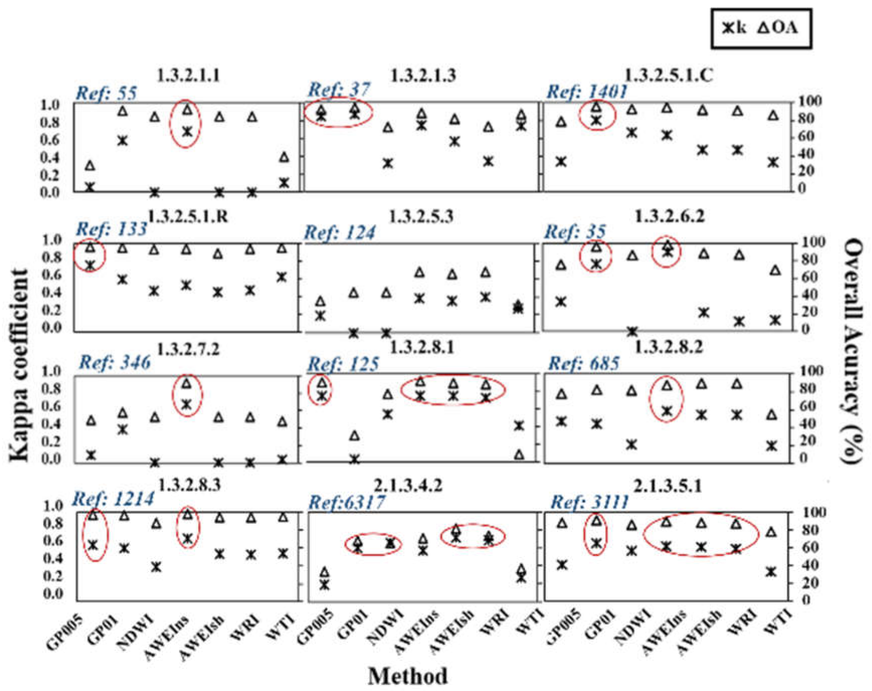
| Lake/Wetland Type | Water Body | Method | Kappa Coefficient | Overall Accuracy (%) | Total Error (%) |
|---|---|---|---|---|---|
| 1.3.2.1.3 | Laguna del Arquillo (4) | GP-0.05 | 0.9 | 92 | 17 |
| GP0.1 | 0.9 | 94 | 16 | ||
| 1.3.2.5.1.C | Laguna Salada de Zorrilla (5) Laguna de El Hito (7) | GP0.1 | 0.8 | 95 | 16 |
| 1.3.2.6.2 | Laguna de los Capellanes (11) Laguna de Alcaparrosa (12) Laguna de Judes (13) | GP0.1 | 0.8 | 96 | 10 |
| AWEInsh | 0.9 | 98 | 5 | ||
| 1.3.2.7.2 | Laguna de Talayuelas (16) Laguna Grande de la Puebla de Beleña (17) | AWEInsh | 0.7 | 92 | 10 |
| 1.3.2.8.1 | Laguna de Fuentillejo (19) | GP-0.05 | 0.8 | 90 | 14 |
| AWEInsh | 0.8 | 92 | 10 | ||
| AWEIsh | 0.8 | 89 | 14 | ||
| WRI | 0.7 | 88 | 16 | ||
| 1.3.2.8.3 | Laguna Blanca de Armagasilla (22) Laguna de Caracuel (23) | GP-0.05 | 0.6 | 97 | 3 |
| GP0.1 | 0.6 | 96 | 4 | ||
| NDWI | 0.4 | 88 | 14 | ||
| AWEInsh | 0.7 | 98 | 2 | ||
| AWEIsh | 0.5 | 94 | 7 | ||
| WRI | 0.5 | 94 | 7 | ||
| WTI | 0.5 | 95 | 5 | ||
| 2.1.3.4.2 | L’Encanyissada (28) Albufera Nueva de Adra (31) | GP0.1 | 0.6 | 87 | 15 |
| NDWI | 0.7 | 86 | 17 | ||
| AWEInsh | 0.6 | 87 | 14 | ||
| AWEIsh | 0.7 | 90 | 12 | ||
| WRI | 0.7 | 88 | 15 | ||
| 2.1.3.5.1 | Salinas de Calp (32) Salinas de Cabo de Gata (33) | GP-0.05 | 0.4 | 88 | 13 |
| GP0.1 | 0.7 | 91 | 11 | ||
| AWEInsh | 0.6 | 86 | 18 | ||
| AWEIsh | 0.6 | 90 | 13 | ||
| WRI | 0.6 | 88 | 15 | ||
| WTI | 0.6 | 88 | 15 |
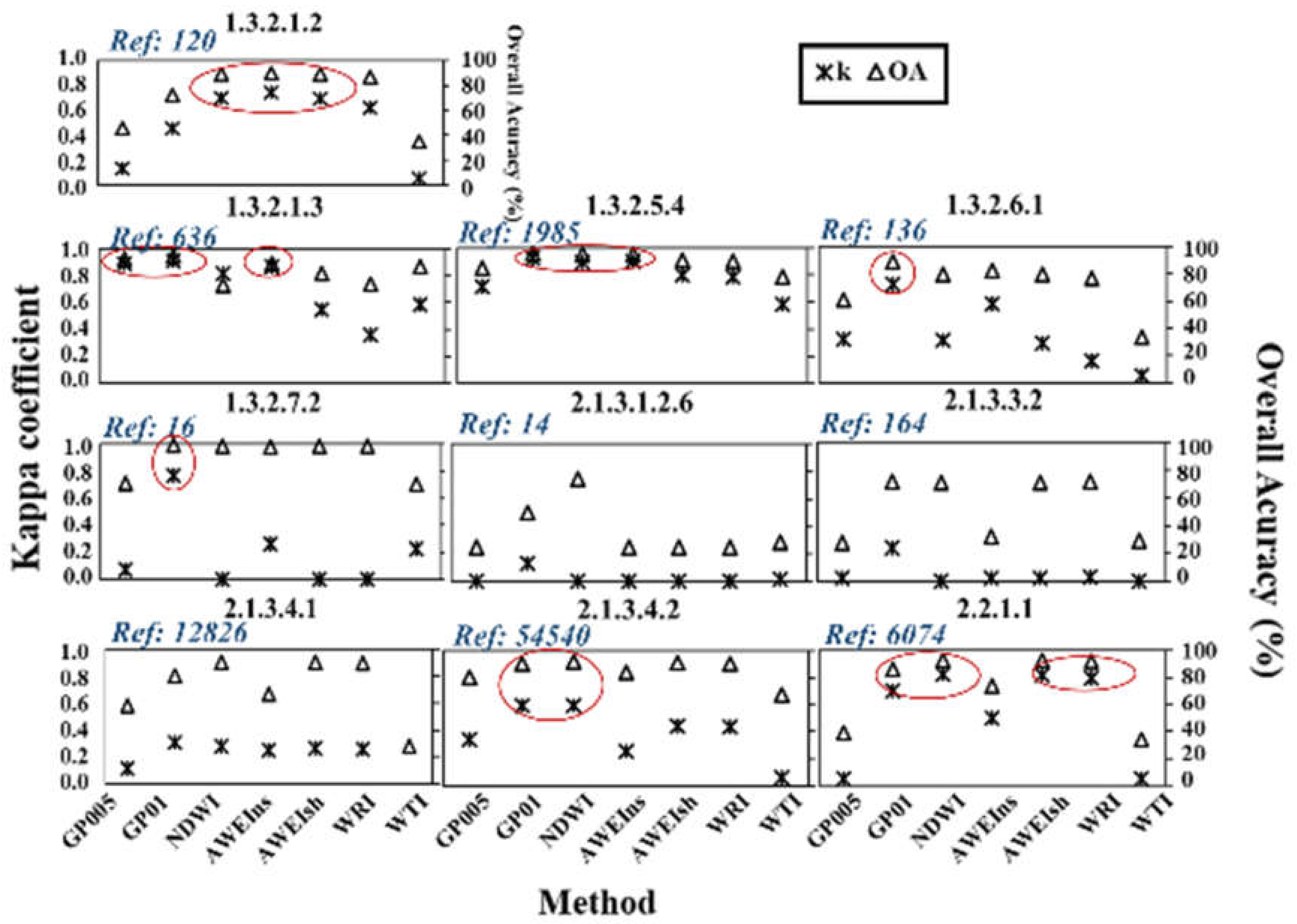
| Lake/ Wetland Type | Water Body | Method | Kappa Coefficient | Overall Accuracy (%) | Total Error (%) |
|---|---|---|---|---|---|
| 1.3.2.1.3 | Laguna del Arquillo (4) | GP-0.05 | 0.9 | 95 | 13 |
| GP0.1 | 0.9 | 96 | 11 | ||
| AWEInsh | 0.9 | 94 | 17 | ||
| 1.3.2.5.4 | Laguna Salada de Chiprana (9) | GP0.1 | 0.9 | 96 | 10 |
| NDWI | 0.9 | 95 | 14 | ||
| AWEInsh | 0.9 | 95 | 13 | ||
| 1.3.2.7.2 | Laguna de Campillo (14) Laguna de Palancoso (15) Charca del Monte (18) | GP0.1 | 0.8 | 99 | 20 |
| 2.2.1.1 | Palmones marshes (34) | GP0.1 | 0.7 | 90 | 20 |
| NDWI | 0.8 | 92 | 20 | ||
| AWEIsh | 0.8 | 92 | 20 | ||
| WRI | 0.8 | 91 | 20 |
Publisher’s Note: MDPI stays neutral with regard to jurisdictional claims in published maps and institutional affiliations. |
© 2021 by the authors. Licensee MDPI, Basel, Switzerland. This article is an open access article distributed under the terms and conditions of the Creative Commons Attribution (CC BY) license (http://creativecommons.org/licenses/by/4.0/).
Share and Cite
Doña, C.; Morant, D.; Picazo, A.; Rochera, C.; Sánchez, J.M.; Camacho, A. Estimation of Water Coverage in Permanent and Temporary Shallow Lakes and Wetlands by Combining Remote Sensing Techniques and Genetic Programming: Application to the Mediterranean Basin of the Iberian Peninsula. Remote Sens. 2021, 13, 652. https://doi.org/10.3390/rs13040652
Doña C, Morant D, Picazo A, Rochera C, Sánchez JM, Camacho A. Estimation of Water Coverage in Permanent and Temporary Shallow Lakes and Wetlands by Combining Remote Sensing Techniques and Genetic Programming: Application to the Mediterranean Basin of the Iberian Peninsula. Remote Sensing. 2021; 13(4):652. https://doi.org/10.3390/rs13040652
Chicago/Turabian StyleDoña, Carolina, Daniel Morant, Antonio Picazo, Carlos Rochera, Juan Manuel Sánchez, and Antonio Camacho. 2021. "Estimation of Water Coverage in Permanent and Temporary Shallow Lakes and Wetlands by Combining Remote Sensing Techniques and Genetic Programming: Application to the Mediterranean Basin of the Iberian Peninsula" Remote Sensing 13, no. 4: 652. https://doi.org/10.3390/rs13040652