PD Steering Controller Utilizing the Predicted Position on Track for Autonomous Vehicles Driven on Slippery Roads


Graduate School of Science and Engineering, Doshisha University, Kyoto 602-8580, Japan
*
Author to whom correspondence should be addressed.
Algorithms 2020, 13(2), 48; https://doi.org/10.3390/a13020048
Submission received: 24 December 2019
/
Revised: 18 February 2020
/
Accepted: 18 February 2020
/
Published: 21 February 2020
(This article belongs to the Special Issue Algorithms for PID Controller 2019)
Abstract
:Among the most important characteristics of autonomous vehicles are the safety and robustness in various traffic situations and road conditions. In this paper, we focus on the development and analysis of the extended version of the canonical proportional-derivative PD controllers that are known to provide a good quality of steering on non-slippery (dry) roads. However, on slippery roads, due to the poor yaw controllability of the vehicle (suffering from understeering and oversteering), the quality of control of such controllers deteriorates. The proposed predicted PD controller (PPD controller) overcomes the main drawback of PD controllers, namely, the reactiveness of their steering behavior. The latter implies that steering output is a direct result of the currently perceived lateral- and angular deviation of the vehicle from its intended, ideal trajectory, which is the center of the lane. This reactiveness, combined with the tardiness of the yaw control of the vehicle on slippery roads, results in a significant lag in the control loop that could not be compensated completely by the predictive (derivative) component of these controllers. In our approach, keeping the controller efforts at the same level as in PD controllers by avoiding (i) complex computations and (ii) adding additional variables, the PPD controller shows better quality of steering than that of the evolved (via genetic programming) models.
1. Introduction
Essentially every year, the demand for autonomously controlled road motor vehicles (hereafter referred to as cars) is rising, and now they could be used both as a taxi [1] or as personal cars. Consequently, the demand for precise control models that provide the safest and fastest transit of the passengers to their destinations is growing. Hereinafter, we consider a control model to be a control feedback mechanism, the description of which we will provide in the following sections. Among the main aspects of such models, the automated control of steering of the car is achieved by continuously adjusting the steering angle of the front wheels of the car. At the moment, the PD controllers are among the most widely used for the steering control of autonomous cars [2,3]. Despite being generally effective under the ordinary dry road conditions and simple to implement, these controllers suffer from several drawbacks. One of them is that, due to the simplicity of structure and low number of variables, they cannot properly cooperate with the physics of the vehicle in the case of a slippery road [2]. When humans drive the car, we dynamically adapt our steering behavior depending on the features of the car (e.g., length, width, mass,) and the road conditions (dry, wet, snowy, etc.) in a way that is difficult to mimic in both PD and PID controllers due to their hard structure with a small number of variables. In addition, the reactivity of these controllers implies that the steering output is a direct result of the currently perceived lateral- and angular deviation of the car from its intended, ideal trajectory. For convenience, here, as in previous studies, we consider the middle of the lane to be the desired ideal trajectory. Because these deviations are used as an error in the error-correcting, feedback control of the steering of the car, the required non-zero value of the error during cornering would result in a trajectory of the car that is always offset to the “outside” of the corner. Consequently, if the turning is initiated as an obstacle-avoiding maneuver, the car will inevitably circumnavigate the obstacle at a distance that is always lower than that of the intended, ideal trajectory, which, in turn, leads to an increased risk of a collision with the obstacle. Moreover, the reactiveness, combined with the tardiness of the yaw control of the car on slippery roads (as a result of the significant reduction of the steering forces—due to the reduced friction coefficient between the tires and the road—that have to overcome the given non-zero yaw moment of inertia of the car) results in a significant lag in the control loop that could not be compensated completely by the predictive (derivative) component of these controllers.
Another challenge of adopting the PD and PID controllers is finding the optimal values of the scaling coefficients of these controllers for the particular road conditions. The optimization of these parameters by human experts often requires extensive knowledge in both the control theory and vehicle dynamics. Automated tuning of the parameters, on the other hand, might require applying heuristic approaches that are notorious with their long runtime even when using a significant computational power [4,5].
In order to address the above-mentioned challenges of the canonical PD controllers, in which the control output is calculated as a weighted sum of the control errors and their derivatives, in our previous research we proposed a PID steering controller featuring an arbitrary (rather than an additive) internal structure, developed heuristically via genetic programming [6].
Another approach to improve the PD controller is adding prediction mechanics. Predictive models were already widely used in application to autonomous vehicles [7] for non-slippery road conditions. One of the most widely used methods is the Model Predictive Control (MPC) [8] and its modifications [9,10]. This method, however, features some drawbacks, which would hinder its applicability to the considered application. One of them is the computational overhead associated with (i) the need to predict too far ahead and (ii) the significant complexity of the predictive model (which would be even greater in slippery road conditions due to the complex nature of the vehicle dynamics of the sliding car).
In this work, we modified the original PD controller by replacing one of the terms with its predicted value. We tried to compensate for the drawbacks of the controller by avoiding (i) adding additional variables and (ii) modifying the structure of the controller that would increase the controller effort. Rather, by using the predicted (instead of the current) value of just one perceived variable, pertinent to the state of the car—the lateral deviation from the center of the road—we demonstrated that the quality of steering of the car on slippery roads could be significantly improved with the same set of perception information of the controller; yet, assuming the availability of the map of the road ahead.
2. Materials and Methods
2.1. Environment and the Car Simulator TORCS
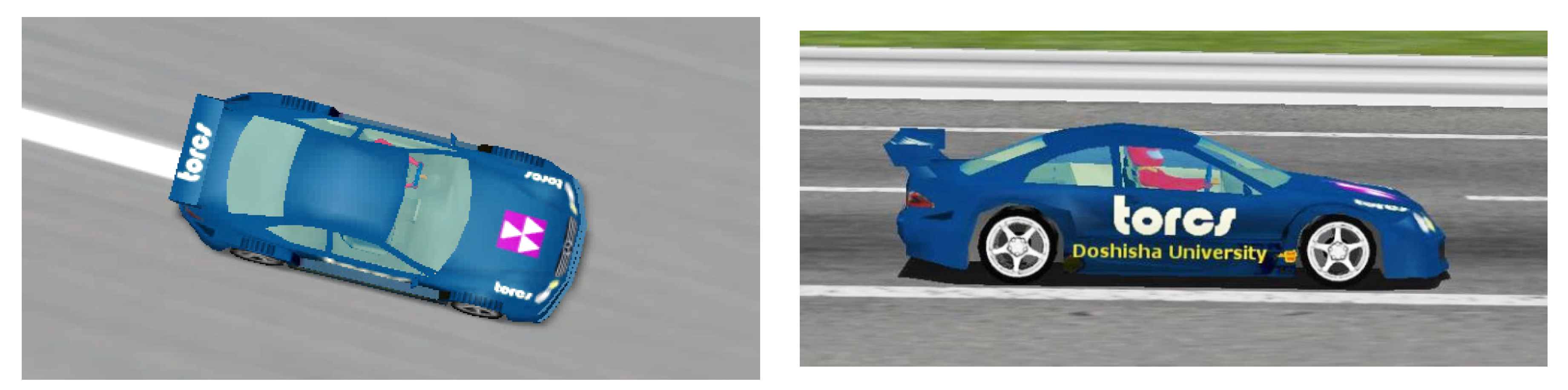
In this work, TORCS [7] was employed to perform a simulation of the experiments. This tool provides an accurate simulation of both the physics environment and mechanics of a car (engine, etc.). For the experiments, a racing model of a rear-wheel-drive car of the Mercedes brand was used, and a list of its parameters is shown in Table 1 below, and Figure 1 shows its view during the races.
As we mentioned earlier [6], the choice of TORCS over different alternatives as a simulator in our experiments was also determined by its computational efficiency, safety, and the availability of its source code.
2.2. The Track
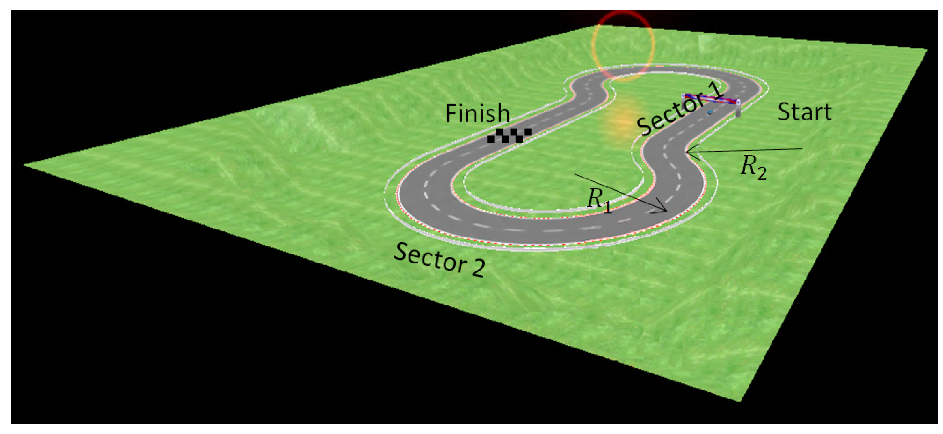
In our experiments, a route called a “fish hook” was constructed (Figure 2). Its length is only 300 m, but its shape contains a straight line, a sharp transition to the left turn, and a long right turn afterward. Such a track belongs to a difficult type of tracks for a human driver.
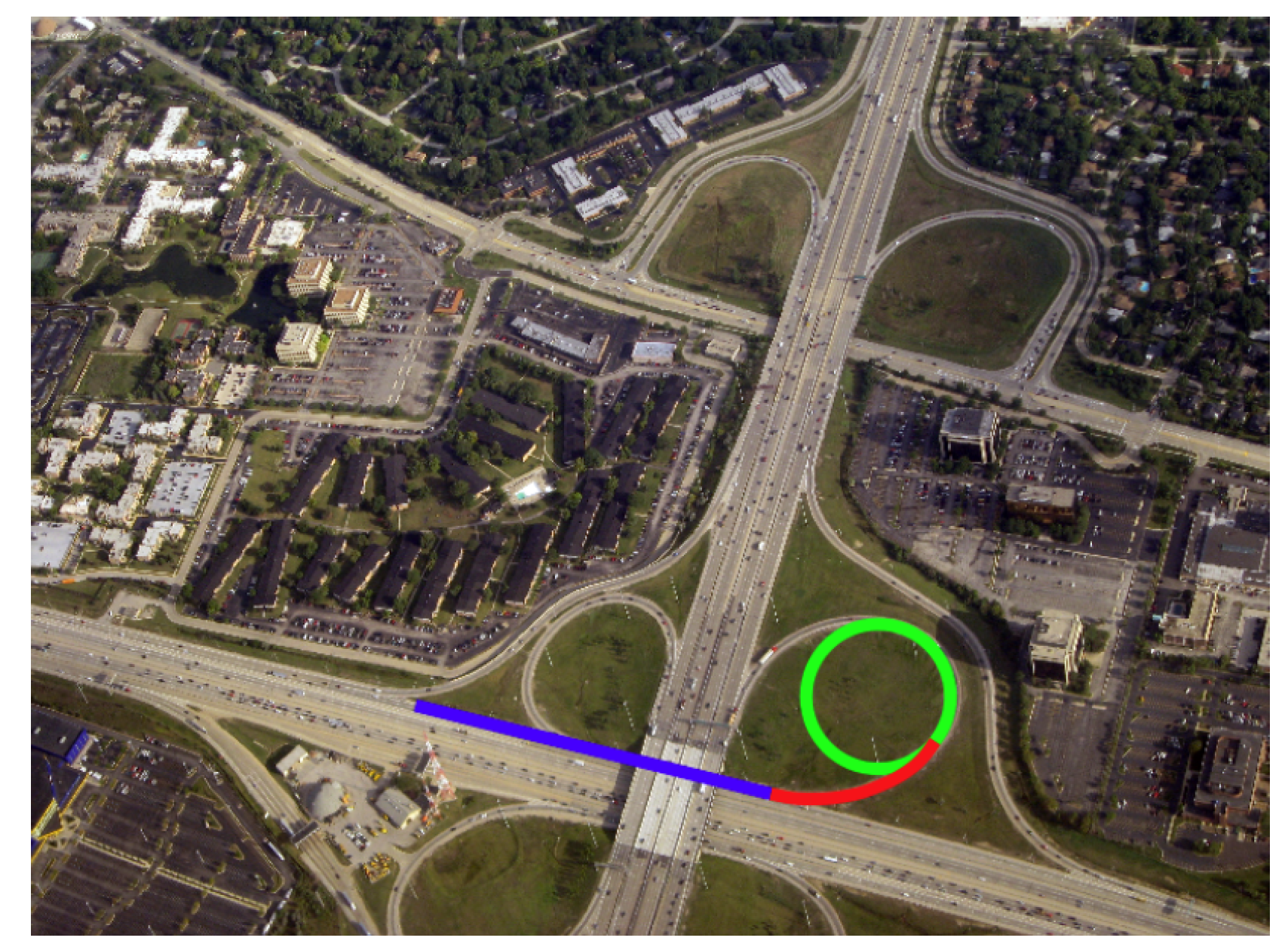
Usually, during the first section of the route—straight—the driver accelerates and, at the maximum speed, begins the passage of the turn. The peculiarity of this rotation is that it does not contain a transition spiral curve part between the straight and the rotation sections. A spiral curve is a geometric element that can be added to a regular curve and provides a gradual transition (red part in Figure 3) from movement in a straight line (blue part in Figure 3) to movement along a circle (green part in Figure 3).
A sharp transition from a straight line to a turn results in stability losses, which, if the track is slippery, may cause an accident. The spiral provides a transition zone, where the driver slowly turns the steering wheel, lateral acceleration slowly increases when entering the spiral or slowly decreases when exiting the spiral and stability is not lost. Such spiral transitions were originally introduced on the railways for safety reasons. They were also implemented on highways in recent years. The mathematical form of the spiral varies [8]. One of the common forms is the Euler or clothoid spiral [9]. In India, the usual transition curve is a hyperbole third-order, and in Germany, autobahns are designed as a continuous series of linked clothoids without tangential sections or circular curves [10]. In the proposed study, the track did not have such transitions. We did this in order to achieve maximum generalization.
In our set of experiments, we did a car runs on the flat road without height changes. Parameters of the track are shown in Table 2. Also, for the experiments, we varied three types of slippery conditions and friction µ between the tires of the car and the surface of the track: rain (µ = 0.5), rain and snow (µ = 0.3), and ice (µ = 0.1).
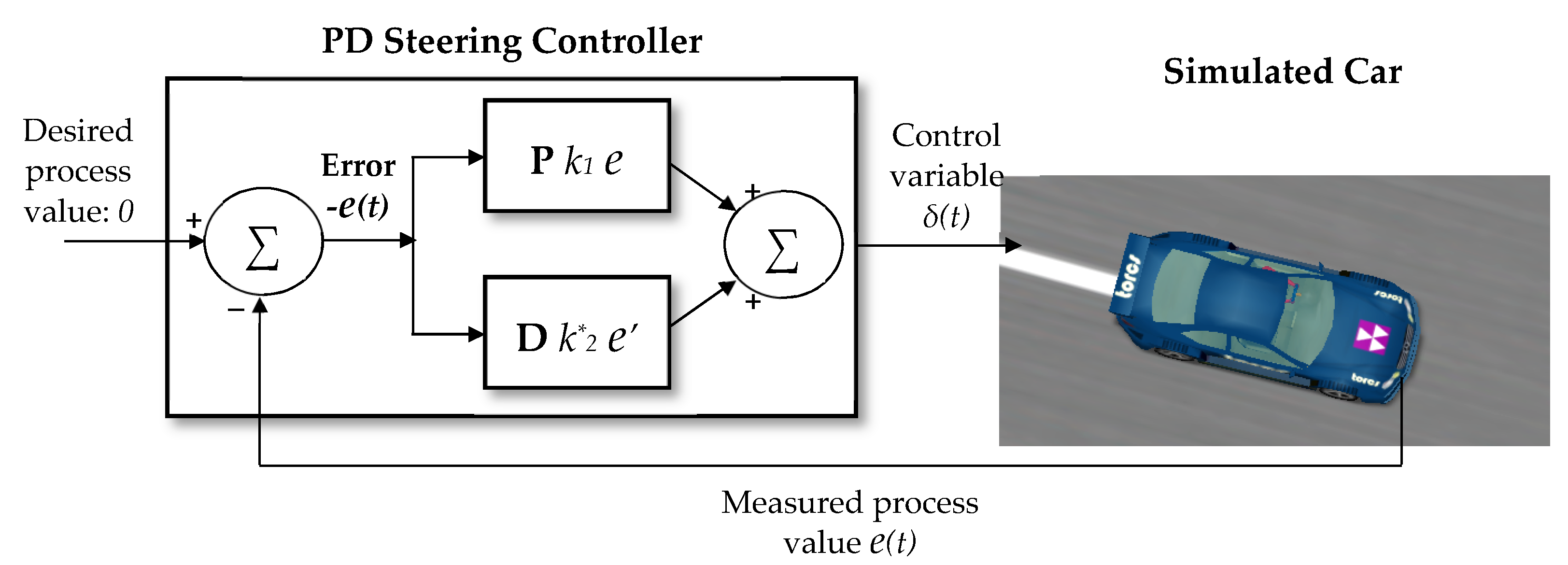
2.3. Servo Control as a PD Controller
In our earlier studies, we showed that the canonical well-known servo control (Figure 4) is a variation of the PD controller. To avoid repetition, we give here only the main statements; the details can be found in our paper [6].
The steering angle defined by this model is a linear combination of scalable deviation from the desired trajectory parameters—the distance e and angle θ shown in Figure 5. The SAF (steering angle function) of the servo control model could be expressed as the following Equation (1):
where δ is the steering angle, and the optimal values of the scaling coefficients (gains) k1 and k2 have an impact to the main requirements to the steering [11]—smoothness, fast response, and stability in the way the car returns to the center of the lane after it deviates from it. These parameters could be chosen from the steering lock angle restrictions in in different ways depending on the specific conditions and features of the road [4].
δ = k1 e + k2 θ
For small angles θ and very short periods of time dt:
θ ≈ de⁄dx = de⁄(V dt)
For constant speed V, Equation (2) could be rewritten as:
θ ≈ kv de⁄dt = kv e’
Applying simple mathematical transformations, we can represent Equation (1) in the following shape expressed the servo-control model of steering as a PD controller:
where e’ is the first derivative of the lateral deviation of the car from the center of the lane. From the PD controller point of view, servo control model represents by itself a closed-loop system. The input—measured process value is equal to the absolute value of the error e—the deviation of the car from the center of the lane. Its output—the control variable—the steering angle δ, is a sum of the proportional (P) and derivative (D) terms of the error. The controller attempts to minimize the value of the error by constantly adjusting the steering angle δ, which, presumably, would yield a trajectory as close as possible to the center of the lane.
δ = k1 e + k2 (kv e’) = k1 e + k*2 e’
2.4. Extending the Servo-Control Model: A PD Steering Controller with Prediction
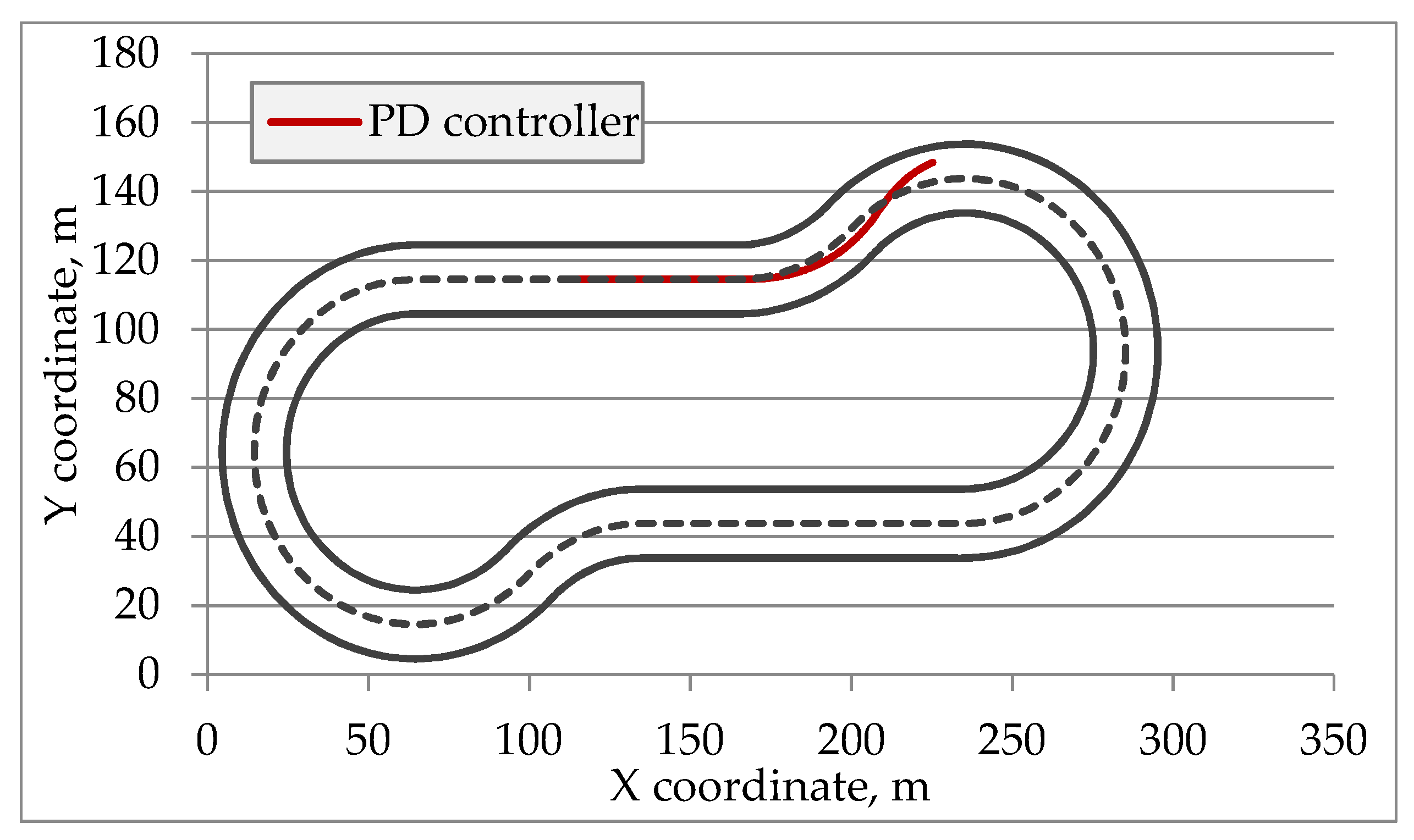
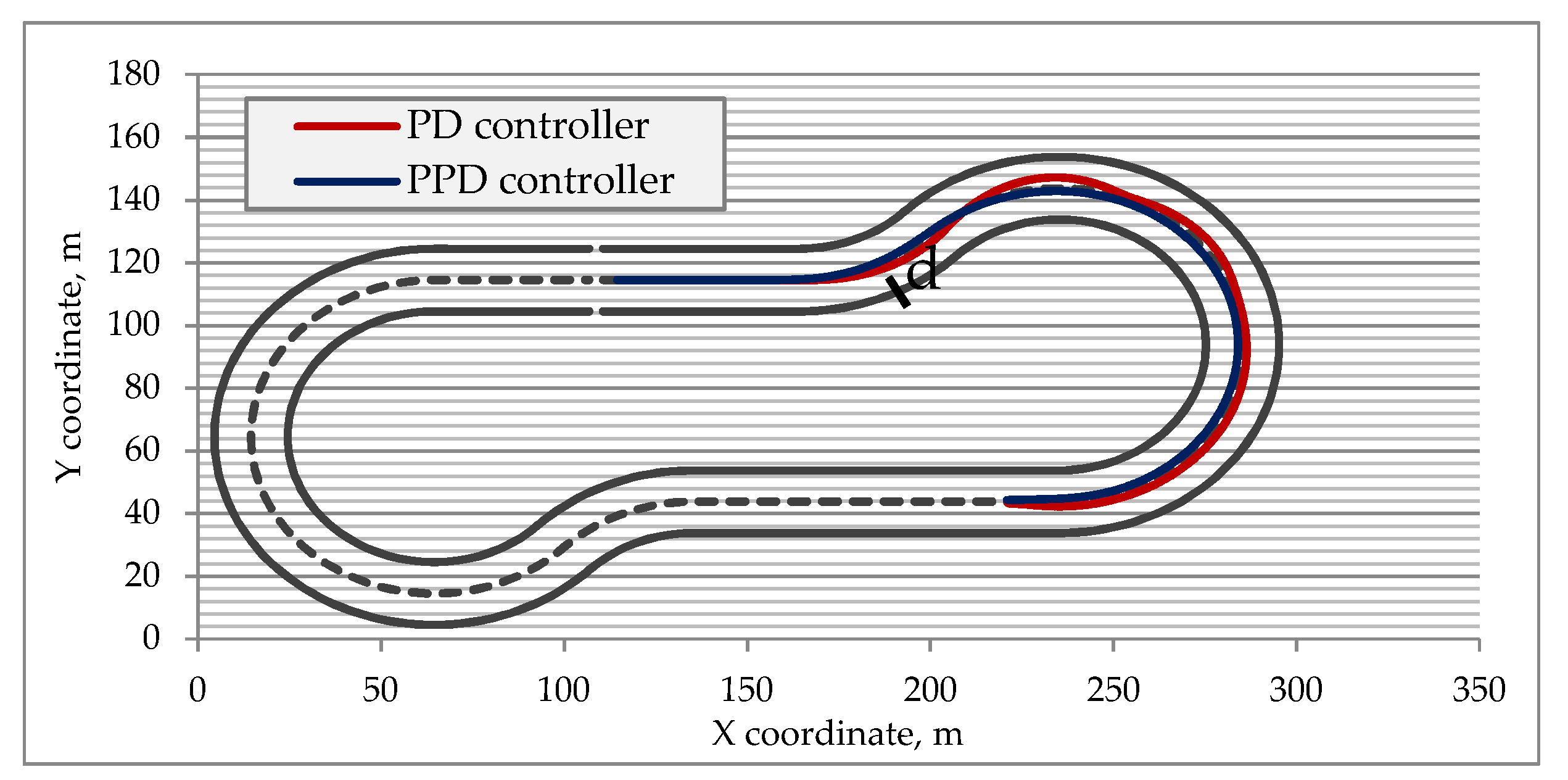
The main common disadvantage of both PD controllers is lagging. It results in an even worse effect on the slippery road. In addition, many real-world physics effects are not taken into account in the controller equations. In practice, these disadvantages lead to the late entrance to the turn, attempts to return to desired trajectory, oversteering and disadvantageous position at the start of second turn, exiting, which could only result in consecutive course deviations, as demonstrated in Figure 6.
While the second disadvantage was already addressed in previous research [6], we did not manage to find sources regarding the first one.
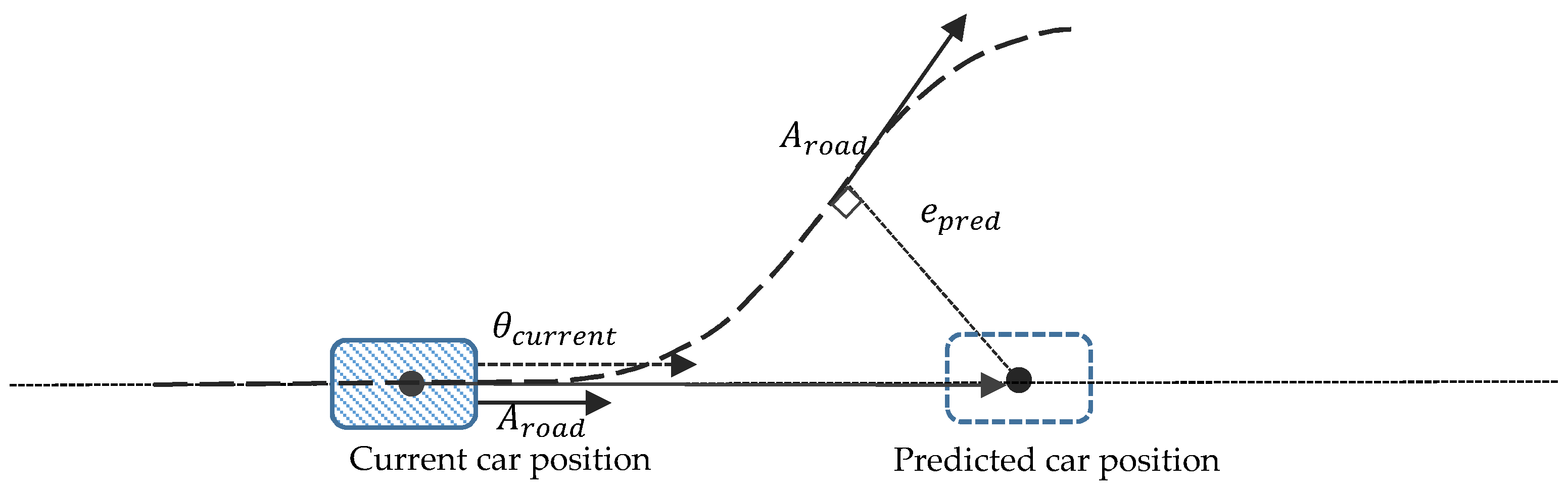
The vehicle position could be predicted using current velocity (Figure 7; Figure 8):
where θ is the angle between the car direction and the road, and epredicted is the distance between the predicted car center and the road calculated by the following Equations (5)–(9):
Here, and are predicted coordinates of the position of the car, is the angle of the road at the point that is closest to the car, F is the function calculating the distance between the car and the center of the lane, , is the speed of the car, and its two orthogonal components, respectively, . is the predicting time interval, and α is the angular deviation of the car from the center of the lane.
This controller we called Predictive PD controller (PPD controller).
It seems natural to also predict the yaw angle. However, it was not performed in our experiments. The reasons for this are not only atomicity of changes that facilitate development and analysis, but the aspiration to achieve human-like behavior of professional and experienced drivers. In contrast to the canonic controller, drivers often use the future position prediction for steering. According to the research [12], having to deal with a lot of information, the human brain experiences cognitive pressure with high speed, which results in a decrease of field of view. In such conditions, it has to operate only the prediction of the position, not the yaw angle. On the other hand, such limitations of human perception do not limit researches in the development of probably more precise models, which predicts both parameters. Nevertheless, such investigations are left for further research and, here, we were curious about how much a change of the value of one of the parameters will affect the quality of driving. We elaborate on this in the discussion section of the paper.
2.5. Steering Controller Obtained by Genetic Programming (GP)
To achieve a more thorough and complete analysis of the new controller, in this paper, we also presented the results of experiments conducted with the previously obtained model with an extended set of parameters and relaxed structure, evolved via a genetic programming (GP-RMEP) [6] method.
The GP approach allowed us to construct a controller of arbitrary complexity and structure, which showed results significantly superior to the canonical PD controller [6]. It took a lot of time at the stage of evolution to build a control equation that would demonstrate good results simultaneously in different environmental conditions, but the resulting model showed good results in terms of vehicle speed during the race and quality of the trajectory. However, as it turned out, this model also has its drawbacks; in particular, it produces frequent oscillations of the steering wheel, which, in the long term, can cause mechanical damage similar to what race cars get. Although this is not a critical flaw, it encourages us to continue research in this area. To avoid self-repetition, we present here in Table 3 only its main parameters, while our previous work contains the details [6].
2.6. Target Quality Function Evaluation
The target quality function value is intended to estimate the quality of the steering produced by the obtained SAF. We defined the criteria of such a quality from the desired characteristics of the trajectory of the car during the trial. It is simulated on a given test track (as shown in Figure 2) featuring a given friction coefficient µ, as follows: first, the simulated car is initially positioned at the starting position of the track. Then the car accelerates slowly to a given target speed. In order to render the task of controlling the car challenging, but solvable, the target speed was constant (maintained by simulated cruise control), and equal to 0.85, 0.9, and 0.95 of the critical speed VCR. The critical speed VCR is the speed at which the car theoretically could pass the turns of the test track with the given coefficient of friction without losing control, running off the track, and eventually crashing. This speed is approximated as the speed at which the centrifugal forces during a steady-state cornering [13] become theoretically equal to the friction force. At the traveling speed of 0.85 of VCR, the car inherently suffers from intermittent instability (due to the yaw inertia both in the entry and exit of corners, and due to dynamic lateral weight transfer in corners [3,7]) that we intend to counter by the use of the obtained SAF. The car, traveling at VCR (or above) is theoretically uncontrollable. Consequently, there would be no existing SAF that results in a steerable car. Similarly, a car traveling considerably slower than VCR does not suffer from any instability, and its steering could be accomplished adequately by the canonical servo-control models. The speeds of the car during the trials on the track with different friction coefficients are shown in Table 4.
The speed of the car is kept constant during the trial by a simple, handcrafted cruise control mechanism that maps the difference between the desired speed (e.g., as shown in Table 4, 13.3 m/s for the trial on a track with friction coefficient µ = 0.5) and the actual one into an increment (or decrement) of the position of accelerator pedal. As the car reaches the desired speed, the steering of the car is assumed by the obtained SAF. Then, the latter starts to continuously (with a sampling frequency of 40 Hz) produce the desired steering angle δ calculated for the currently perceived values of the parameters pertinent to the state of the car. The desired trajectory of the car is the center of the lane. The estimation of the current trajectory obtained via the SAF with new parameters is calculated with the same target quality function as earlier [4] with the purpose of a correct result comparison.
According to this, the target quality function F is a weighted sum of the following two components: (i) the area AT under the trajectory of the car around the center of the lane (as an integral of the absolute value of lateral deviation e) and (ii) the average of the lateral velocity VL_AVR (as an integral of the lateral acceleration a) of the car:
F = AT + CV VL_AVR
We would like to note that for different steering tasks, we might need to keep track of both components of the target quality function of obtained SAF separately (and to implement a two-objective optimization [14]) instead of fusing both these components in a single scalar value. This would allow us to obtain a set of Pareto-optimal SAF that features different combinations of the area under the trajectory of the car and the average of its lateral velocity. SAF featuring a wide area under the trajectory might be needed in a slow and comfortable lane change on a low-traffic highway. On the other hand, the SAF that results in oscillating trajectories with higher lateral accelerations might be needed to safely circumnavigate suddenly appeared obstacles. However, for the given task, the proposed evaluation of the target quality function is sufficient.
3. Experimental Results
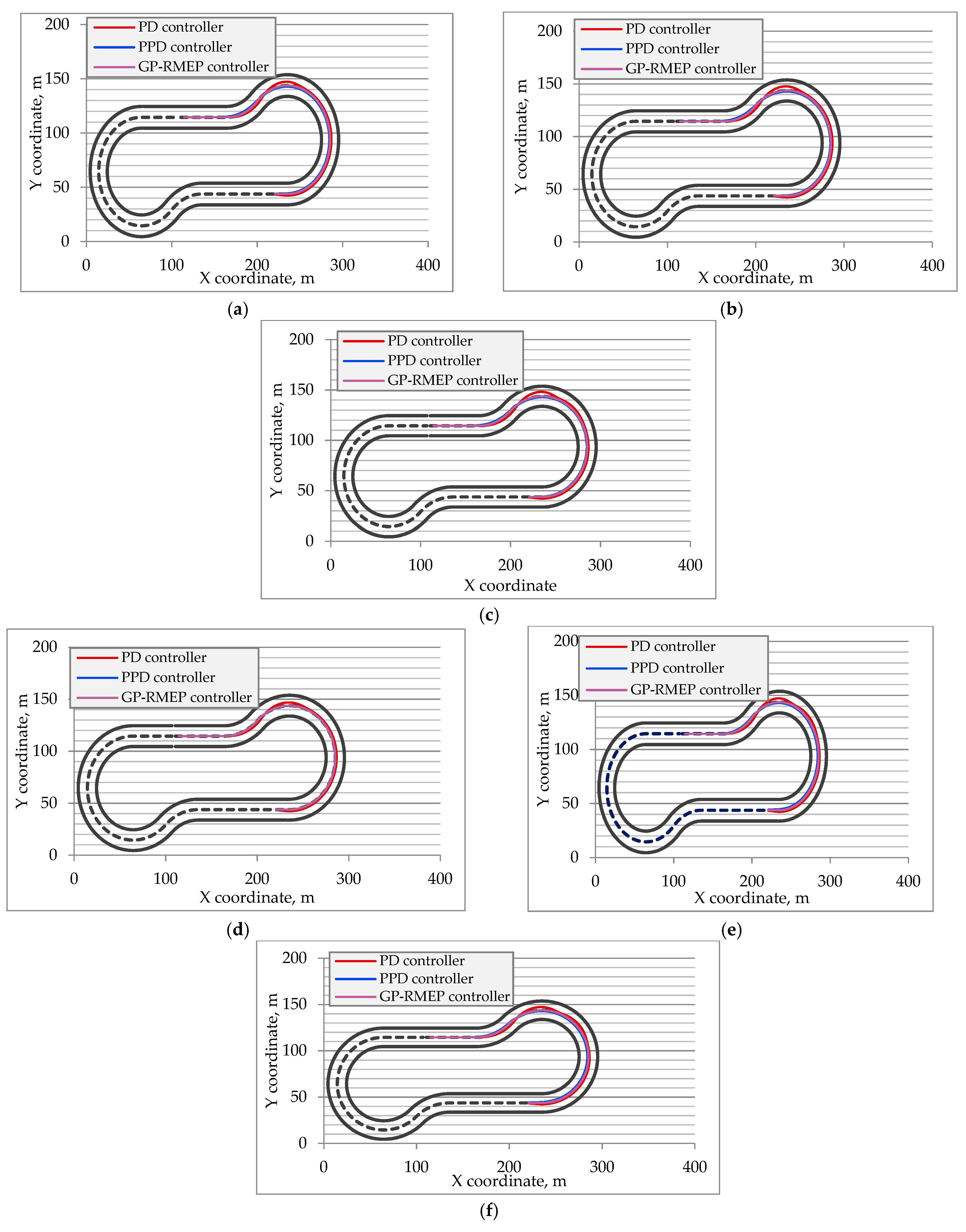
For each road condition described in Table 4, we developed a new analytic equation and tested them with different levels of target speed. We pick optimal parameters for a PD controller according to algorithms in our previous work [6] to optimize its quality function and controller perception. So, we ran simulations for predictive PD, best PD, and, constructed via genetic programming [7], GP-RMEP controlling models. Algorithms were designed for the same track with the same conditions and the same estimation quality function F, so we could compare them. Resulting car trajectories are presented in Figure 9.
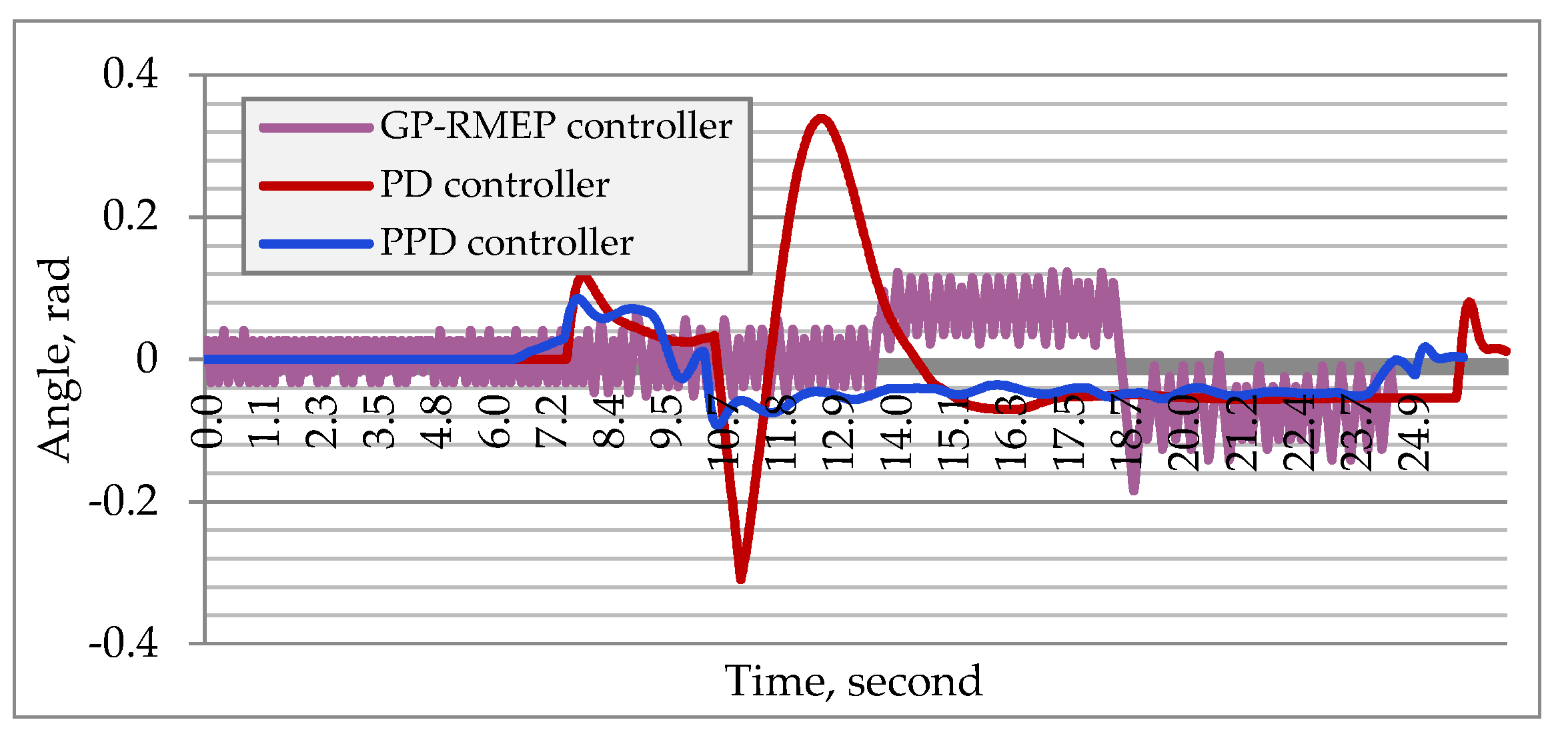
As Figure 9 illustrates, under each road condition, the trajectory provided by the PD controller version with prediction was better (i.e., closer to the center of the lane). In Figure 10, the changes of steering angle for parameters , is shown. It could be noted that the new controller provides smooth steering, similar to the PD controller but with lower amplitude. This characteristic also corresponds to driving stability. We analyzed the smoothness of each function as a number of sign changes in the approximate first derivative: . The results were as follows: GP-RMEP—349 changes, PD controller—218 changes, PPD controller—98 changes. This PPD controller is more stable than PD and has lower angle change amplitudes. As for comparison with the GP method, the high frequency of oscillations makes them less influencing but exhausts the tires and mechanical parts of the steering. We compared their target quality function values, and the results are shown in Table 5.
As the results shown in Table 5 demonstrate, the PPD controller outperforms the PD and is comparable with the GP-RMEP controller in terms of target quality function. Thus, the new controller has a trajectory close to the best trajectory obtained with the GP controller but does not have oscillations that could lead to mechanical damage [15]. Since, according to our earlier studies [6,13], oscillations in the GP-RMEP method are part of its tactics aimed at increasing and maintaining the largest slip angle on tires and, accordingly, cannot be removed from the method without reducing the speed and safety of the car, the result we obtained, which is close in quality to GP-RMEP and free from oscillations, is an important result for us.
Also during the analysis of the proposed model, we discovered several features, as described below.
3.1. Time Needed to Return on Desired Trajectory
The first feature is a more rapid return to the center lane. As shown in Table 6, in each considered case, the time needed to return on the desired trajectory decreased by 4% to 11%, which corresponds to 10-20 m of movement with speeds from Table 4 and could be crucial for safety.
These times demonstrate how fast the vehicle returns from the position occupied while being affected by the forces during the turn. The parameter is directly related to the safety of a driver. Large values could correspond to both a noticeable distance to desired trajectory or inconvenient vehicle orientation. Both cases may cause the following complications, resulting, for instance, in a turning vehicle in oncoming traffic.
3.2. Critical Speed Rising
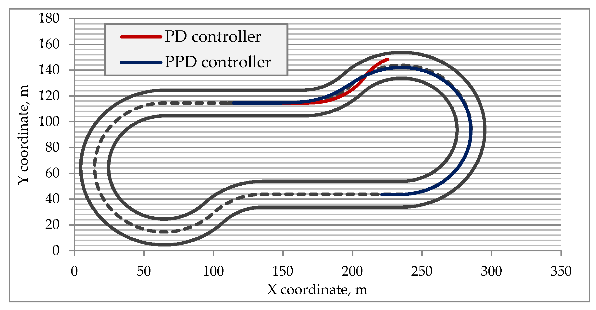
Another feature of the proposed approach, which improves safety, is demonstrated in Figure 11. Here, with identical environment parameters, the vehicle without prediction, moving at a speed above critical, loses control and crashes, while the model with prediction successfully finishes the race. The reason for this results from differences in trajectories. As it was shown in previous studies [6], the vehicles’ critical speed during the turn is proportional to . The model with prediction starts the turn earlier, which results in increased R, and as a result, increased critical speed. In target quality function, this should lead to improvements in the parameter, corresponding to the car stability—second addend in Equation (10). This is covered in the Discussions Section in Table 7.
3.3. Safe Distance
The third feature is increased distance to potential obstacle during the turn, i.e., the moment of the minimal stability of a car (Figure 12).
Due to prediction, the vehicle starts the turn earlier. This not only makes the trajectory smoother and increases turn radius but also allows avoiding potential causes of turn—road twist or unexpected obstacle. According to data from Table 7, the average distance to an obstacle increased by 35%.
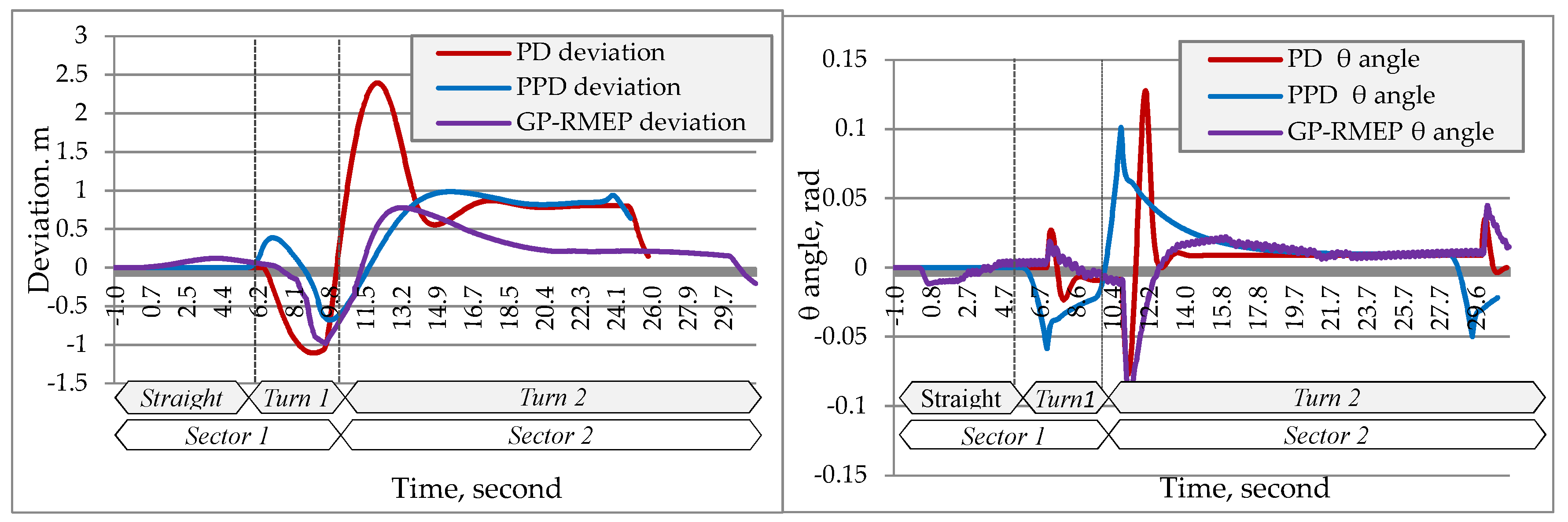
These numbers, as well as the values of the target quality function, indicate the remoteness of the results occurred by each method from the desired ones (if they were equal to zero, the car would move along the chosen trajectory without deviations caused by instability). In other words, these numbers could be interpreted as the error amount of methods. Figure 13 demonstrates distance and angle errors for all compared methods. In these terms, PPD performs better than PD and has similar changes of amplitudes with the GP-RMEP controller.
4. Discussion
Data from Table 8 demonstrate that improvements of a new model affected both target quality function addends—deviation from the trajectory and lateral acceleration. An increase of one of the parameters may lead to the decrease of another. The closer the vehicle is to the center of the lane, the stronger the forces affecting it during the turn. However, in this case, the new model demonstrated improvements in both parameters, so called non-zero sum, which indicates qualitative model enhancement in contrast to parameter tuning.
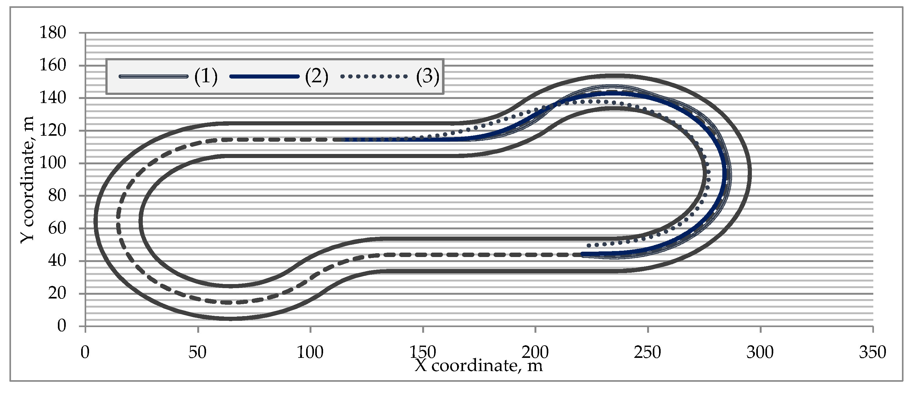
Another issue that was not covered previously is the value of prediction time distance. In other words, it is the task of finding the optimal parameter for Equations (7)–(9). Previously, the value was chosen manually for each configuration and was in the range [0.8…1.8] seconds. Too short of a prediction time does not allow achieving the effect described in Section 2.4 and leads to trajectory Type (1) in Figure 14. In contrast, too long of a period provides changes to the trajectory, which makes it too far from that desired, as shown on Trajectory (3), Figure 14.
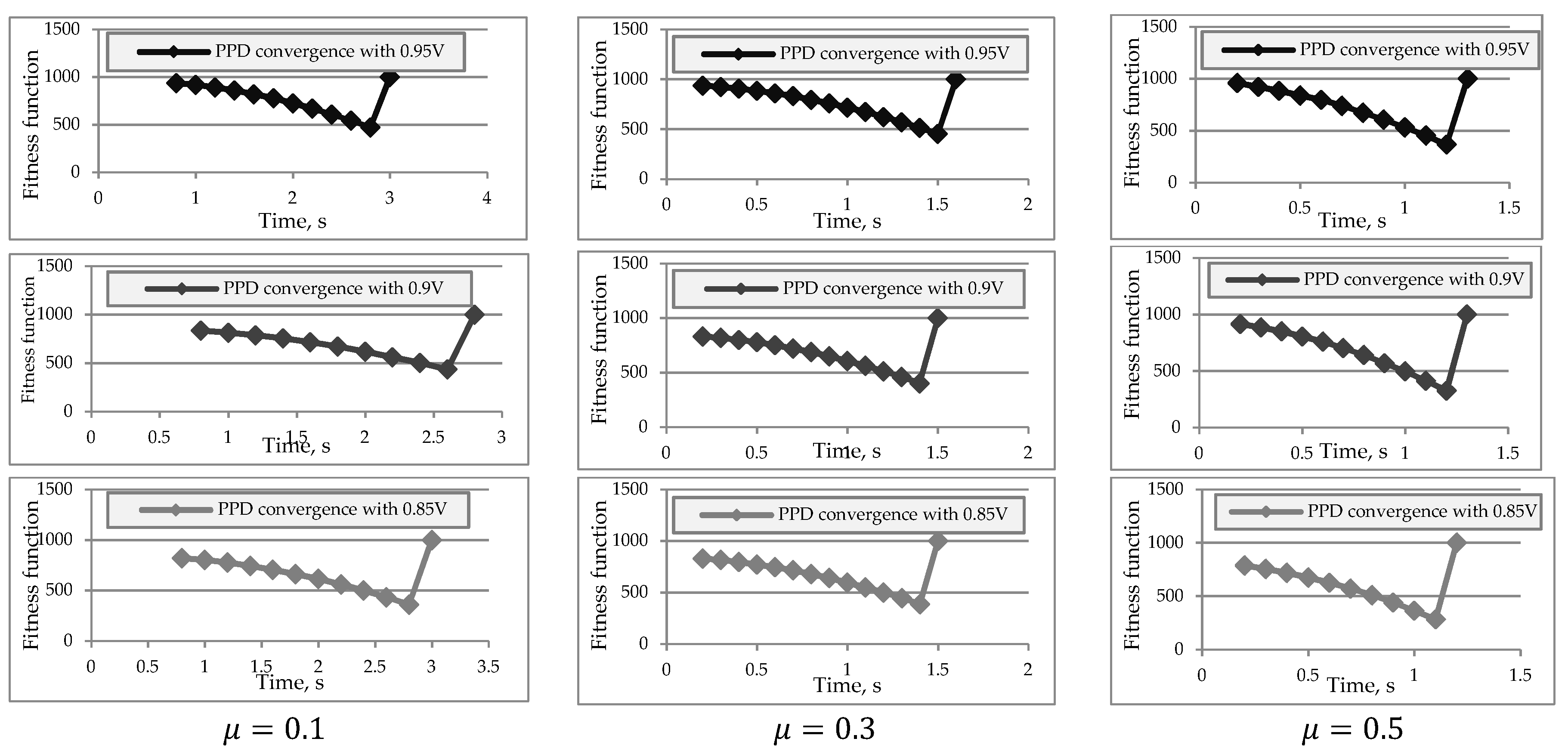
Therefore, we ran a series of experiments in order to find the optimal value of this parameter. Figure 15 shows the results. We started the search from the small prediction times provided trajectory (1) and increased the time value until the result become equal to 1000 (which means the car crashed). The optimal values of prediction time could not be less than what we start from because they will turn into the PD controller results, and they could not be more than those that lead to the car crash already because of its remoteness from reality. We also note that an increase of target speed along with a decrease of friction coefficient increases the optimal prediction time. In other words, under less stable conditions, the prediction should be farther.
Another thought that we mentioned before in the Introduction Section is a special form of the safe trajectory that has a linear curvature profile, which is comfortable for the turning car with high speed.
In order to compare the obtained by PPD controller trajectory shape with clothoid, we combined them on a single plot. Clothoid could be constructed by solving the system of differential equations below, called the “reconstruction equation”.
A clothoid is uniquely defined by:
- Coordinates and heading at which it starts: ();
- Its length L;
- Its linear curvature function, which is determined by the two coefficients ().
With these five values (), we can evaluate the clothoid’s position and heading (x(s), y(s), (s)) at any point s in area [0; L]. We did that by solving the following equations:
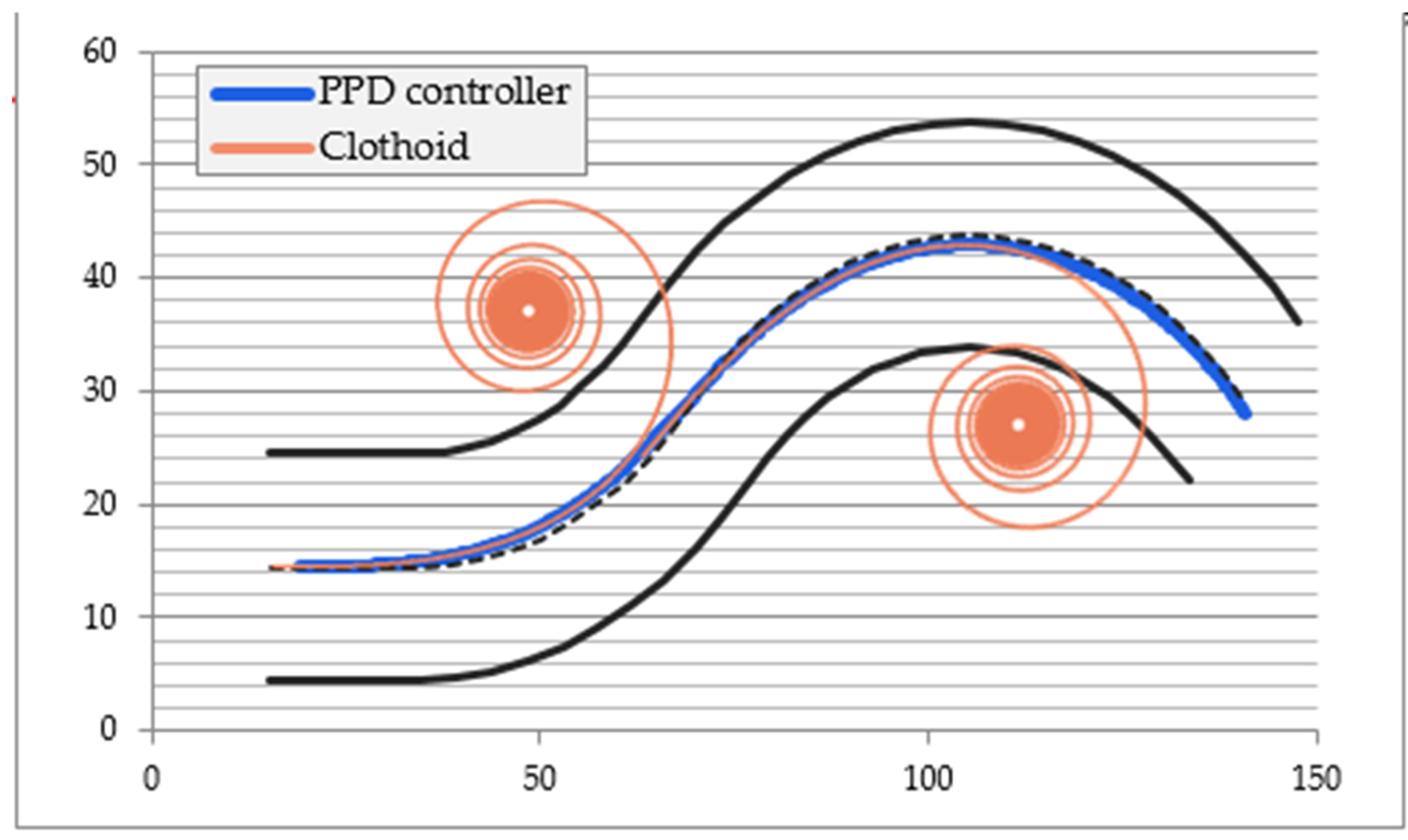
Now, in Figure 16, we can see that our new model produces a trajectory that has a very similar shape to the clothoid (0, 0, 0, 100, 0, 0.1), which was turned around the center.
According to the researches [16], the best and smoothest transition curve to be used as a section of the path is the clothoid. The fact that the PPD controller we developed approached the same conclusion with its results, along with their comparison with the results of other controllers, once again indirectly indicates the effectiveness of the new controller.
5. Conclusions
We researched and implemented the predictive PD controller in the TORCS simulator environment for the race car model (Mercedes CLK). In spite of the fact that we tested a car with specific parameters (a race car), providing, among other things, greater stability (for example, the height of its center of gravity is lower than usual), some of the found features and control tactics can be applied to regular cars. The height of the center of the gravity—together with the lateral forces—would determine the amount of the lateral weight transfer of the car on cornering, which, in turn, would affect the distribution of the normal forces on the tires. On slippery roads, due to the lower lateral forces applied to the cornering car (due to the lower friction coefficients), we assume that the lateral weight transfer would be negligible, regardless of the height of the center of the gravity of the car. This controller relies on the predicted position of a vehicle instead of the current position. The several series of experiments confirmed the relevance of the applicability of such an approach in practice. In fact, the new model demonstrated not only better results but also more native and adequate behavior, which provides greater safety and stability of driving on a slippery road. Based on the reaction style adopted by the human driver to the obstacle that appears in the field of view, this model is able to avoid them by changing its behavior in advance. Depending on the selected speed, the optimal prediction time was computed. During the analysis of the method, it was compared with previously studied methods, which we referred to in this article (PD, PID, GP-RMEP). During the comparison, it turned out that our modification of the PD controller showed results close to those found using genetic programming (GP-RMEP), which demonstrated best adaptability and applicability on slippery roads. The additional studies of this parameter, involving machine learning, are left for further research.
Author Contributions
Conceptualization, I.T.; Investigation, N.A.; Methodology, N.A.; Project administration, K.S.; Software, N.A.; Supervision, I.T. and K.S.; Validation, I.T.; Writing—original draft, N.A.; Writing—review & editing, I.T. and K.S. All authors have read and agreed to the published version of the manuscript.
Funding
This work was funded in part by MEXT-supported Program for Strategic Research Foundation at Private Universities in Japan (2014–2018).
Conflicts of Interest
The authors declare no conflict of interest.
References
- Stone, P.; Brooks, R.; Brynjolfsson, E.; Calo, R.; Etzioni, O.; Hager, G.; Hirschberg, J.; Kalyanakrishnan, S.; Kamar, E.; Kraus, S.; et al. Artificial Intelligence and Life in 2030. In Proceedings of the One Hundred Year Study on Artificial Intelligence: Report of the 2015-2016 Study Panel, Stanford, CA, USA, 6 September 2016; p. 52. [Google Scholar]
- Le-Anh, T.; De Koster, M.B. A Review of Design and Control of Automated Guided Vehicle Systems. Eur. J. Oper. Res. 2006, 171, 1–23. [Google Scholar] [CrossRef]
- Cheein, F.; De La Cruz, C.; Bastos, T.; Carelli, R. SLAM-based Cross-a-Door Solution Approach for a Robotic Wheelchair. Int. J. Adv. Robot. Syst. 2010, 7, 155–164. [Google Scholar] [CrossRef]
- Alekseeva, K.S.N.; Tanev, I. Evolving a Single-variable Controller for Automated Steering of a Car on Slippery Roads. In Proceedings of the SICE Annual Conference 2018: SCIE 2018, Nara, Japan, 11–14 September 2018; pp. 680–685. [Google Scholar]
- Huang, J.; Tanev, I.; Shimohara, K. Evolving a general electronic stability program for car simulated in TORCS. In Proceedings of the 2015 IEEE Conference Computational Intelligence and Games (CIG), Tainan, Taiwan, 31 August–2 September 2015; pp. 446–453. [Google Scholar]
- Alekseeva, N.; Tanev, I.; Shimohara, K. Evolving the Controller of Automated Steering of a Car in Slippery Road Conditions. Algorithms 2018, 11, 108. [Google Scholar] [CrossRef] [Green Version]
- Wymann, B.C.R.; Dimitrakakis, C.; Sumner, A.; Espié, E.; Guionneau, C. TORCS, the Open Racing Car Simulator, v1.3.5. 2013. Available online: http://www.torcs.org (accessed on 20 February 2020).
- Komoriya, K.; Tanie, K. Trajectory Design and Control of a Wheel-type Mobile Robot Using B-spline Curve. In Proceedings of the IEEE/RSJ International Workshop on Intelligent Robots and Systems ‘(IROS ’89)’ the Autonomous Mobile Robots and Its Applications, Tsukuba, Japan, 4–6 September 1989; pp. 398–405. [Google Scholar]
- Marzbani, H.; Jazar, R.; Fard, M. Better Road Design Using Clothoids. In Sustainable Automotive Technologies; Springer: Cham, Switzerland, 2015; pp. 25–40. [Google Scholar]
- Lamm, R.; Psarianos, B.; Choueiri, E.M. A practical safety approach to highway geometric design International case studies: Germany, Greece, Lebanon, and the United States. In Proceedings of the International Symposium on Highway Geometric Design Practices, Boston, MA, USA, 30 August–1 September 1995. [Google Scholar]
- Melder, N.; Tomlinson, S. Racing Vehicle Control Systems using PID Controllers. Game AI Pro 2014, 491–500. [Google Scholar]
- Zeeb, K.; Buchner, A.; Schrauf, M. Is take-over time all that matters? The impact of visual-cognitive load on driver take-over quality after conditionally automated driving. Accid. Anal. Prev. 2016, 92, 230–239. [Google Scholar] [CrossRef] [PubMed]
- Alekseeva, N.; Tanev, I.; Shimohara, K. On the Emergence of Oscillations in the Evolved Autosteering of a Car on Slippery Roads. In Proceedings of the 2019 IEEE/ASME International Conference on Advanced Intelligent Mechatronics (AIM), Hong Kong, China, 8–12 July 2019; pp. 1371–1378. [Google Scholar]
- Coello, C.A.C.; Lamont, G.B.; Van Veldhuizen, D.A. Evolutionary Algorithms for Solving Multi-Objective Problems; Springer: New York, NY, USA, 2007. [Google Scholar]
- Frère, P. Sports Car and Competition Driving; Pickle Partners Publishing: Auckland, New Zealand, 2016. [Google Scholar]
- Marzbani, H.; Simic, M.; Fard, M.; Jazar, R. Better Road Design for Autonomous Vehicles Using Clothoids. In Intelligent Interactive Multimedia Systems and Services; Springer: Cham, Switzerland, 2015; pp. 265–278. [Google Scholar]
Figure 1.
Snapshots of the simulated car.

Figure 2.
Hook-type test track.

Figure 3.
Rotation curve. The transition between the straight part (blue) and circular part (green) is a spiral curve (red). Picture is taken from https://cifrasyteclas.com/clotoide-la-curva-que-vela-por-tu-seguridad-en-carreteras-y-ferrocarriles/.
Figure 3.
Rotation curve. The transition between the straight part (blue) and circular part (green) is a spiral curve (red). Picture is taken from https://cifrasyteclas.com/clotoide-la-curva-que-vela-por-tu-seguridad-en-carreteras-y-ferrocarriles/.

Figure 4.
Servo-control model of steering as a PD steering controller. The steering angle function (SAF), defining the steering angle δ is implemented as a sum of the proportional-(P) and derivative (D) terms of the error—the deviation e from the center of the lane.
Figure 4.
Servo-control model of steering as a PD steering controller. The steering angle function (SAF), defining the steering angle δ is implemented as a sum of the proportional-(P) and derivative (D) terms of the error—the deviation e from the center of the lane.

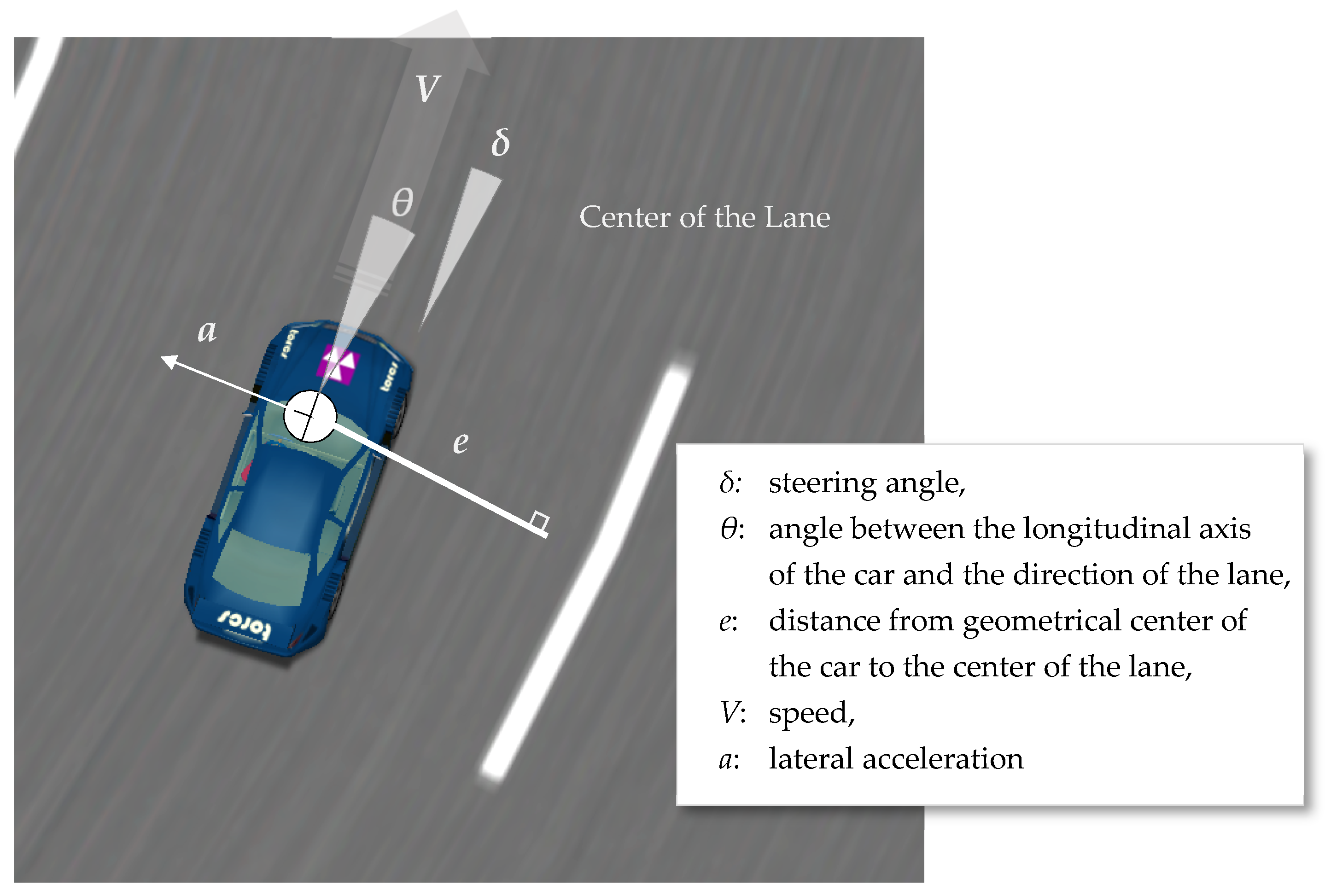
Figure 5.
Most relevant variables pertinent to the state of the car. Variables θ and e are directly involved in the calculation of the steering angle δ according to the servo-control model.
Figure 5.
Most relevant variables pertinent to the state of the car. Variables θ and e are directly involved in the calculation of the steering angle δ according to the servo-control model.

Figure 6.
Tracking of the center of the car on the track during the race with friction 0.1 and . In the highest point of the trajectory, a crash was occurring.
Figure 6.
Tracking of the center of the car on the track during the race with friction 0.1 and . In the highest point of the trajectory, a crash was occurring.

Figure 7.
Predicting the lateral deviation of the car epred.

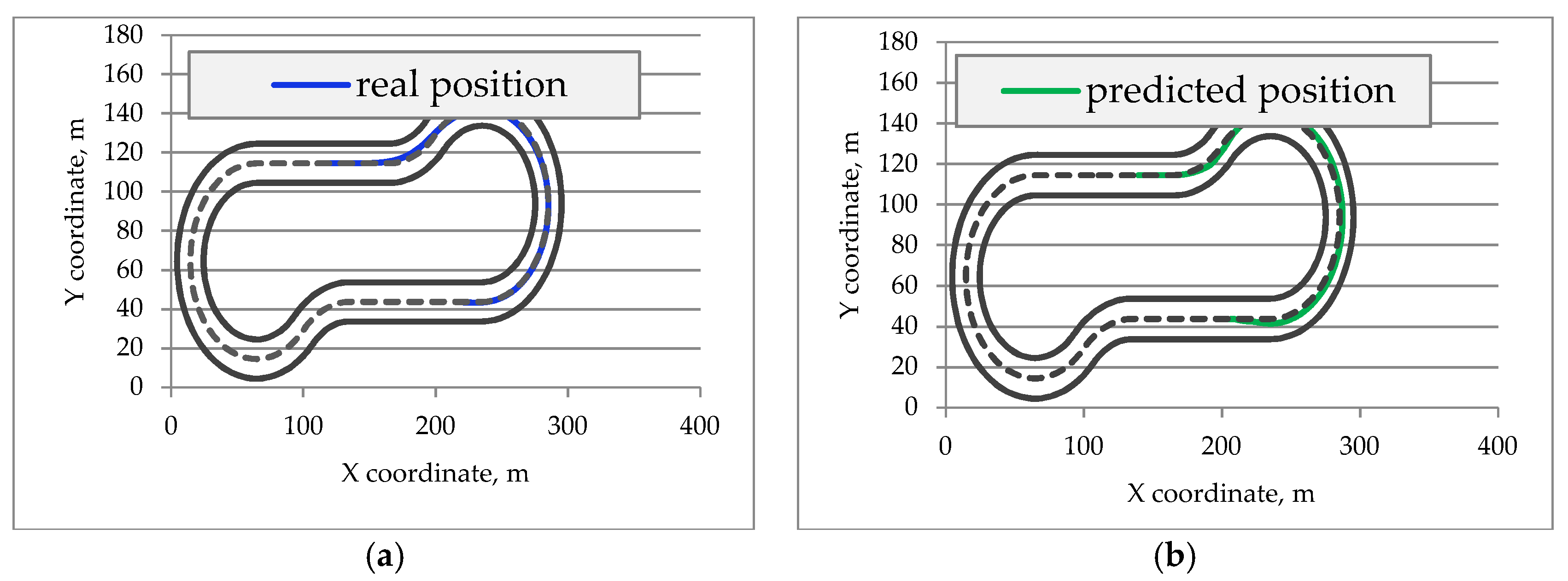
Figure 8.
Real trajectory of the car (a) and predicted position of the car (b). Time of the prediction—1.5 s, = 0.1.
Figure 8.
Real trajectory of the car (a) and predicted position of the car (b). Time of the prediction—1.5 s, = 0.1.

Figure 9.
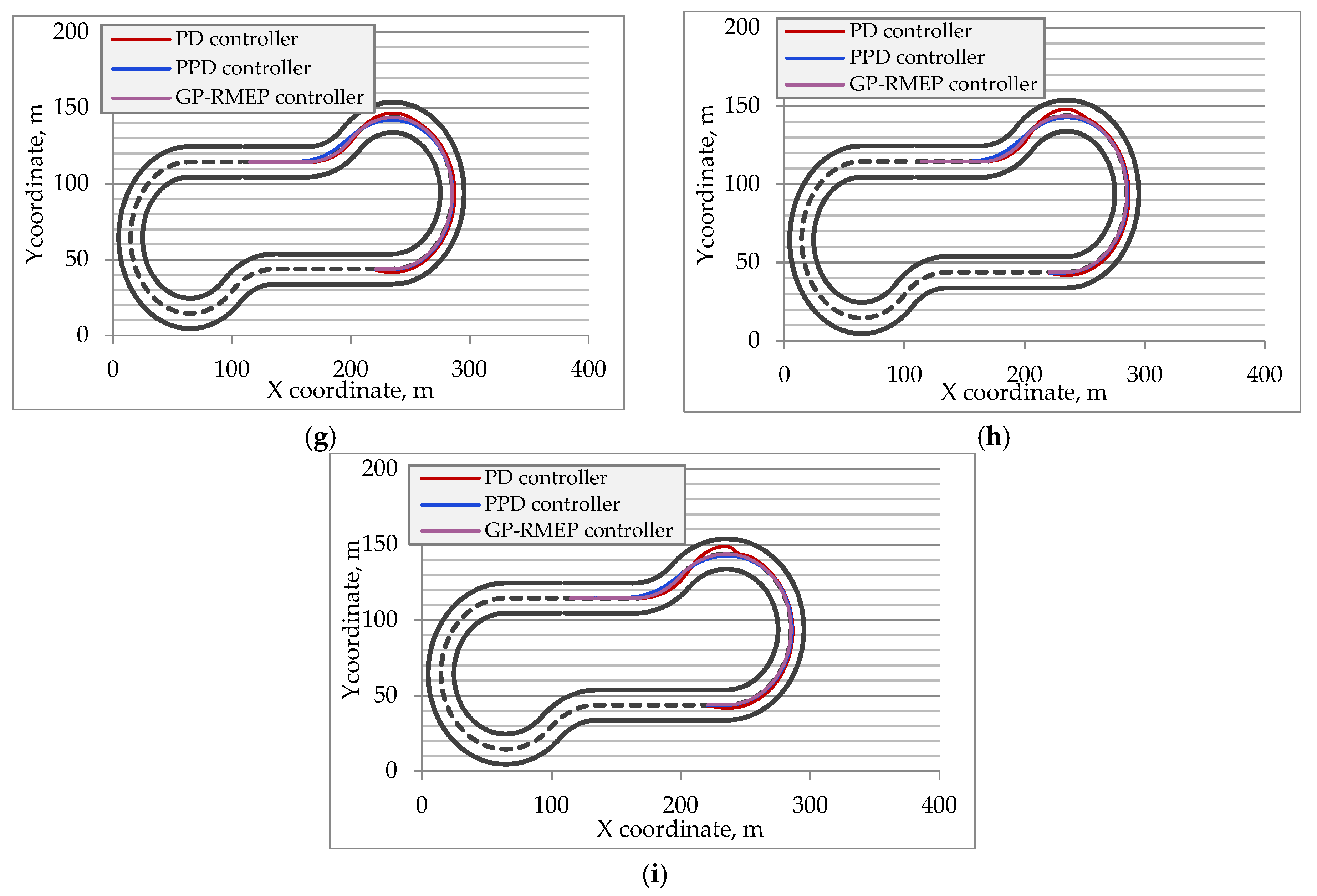
Car trajectories on the track tuned with prediction SAF of standard PD controller for friction coefficients. The purple curves correspond to the GP-RMEP controller, blue curves to the trajectories controlled by SAF with prediction, red curves to the original SAF. (a) 0.5, 0.85 ; (b) 0.5, 0.9 ; (c) 0.5, 0.95 ; (d) 0.3, 0.85 ; (e) 0.3, 0.9 ; (f) 0.3, 0.95 ; (g) 0.1, 0.85 ; (h) 0.1, 0.9 ; (i) =0.1, 0.95 .
Figure 9.
Car trajectories on the track tuned with prediction SAF of standard PD controller for friction coefficients. The purple curves correspond to the GP-RMEP controller, blue curves to the trajectories controlled by SAF with prediction, red curves to the original SAF. (a) 0.5, 0.85 ; (b) 0.5, 0.9 ; (c) 0.5, 0.95 ; (d) 0.3, 0.85 ; (e) 0.3, 0.9 ; (f) 0.3, 0.95 ; (g) 0.1, 0.85 ; (h) 0.1, 0.9 ; (i) =0.1, 0.95 .


Figure 10.
Dynamics of the steering angle for different types of controllers—the controller input is , .
Figure 10.
Dynamics of the steering angle for different types of controllers—the controller input is , .

Figure 11.
Car trajectory on the track tuned with prediction SAF of standard PD controller for friction coefficient µ = 0.1 with target speed equal to . The blue curve corresponds to the trajectory controlled by PPD controller, and red to the original PD controller.
Figure 11.
Car trajectory on the track tuned with prediction SAF of standard PD controller for friction coefficient µ = 0.1 with target speed equal to . The blue curve corresponds to the trajectory controlled by PPD controller, and red to the original PD controller.

Figure 12.
Distance between the car and obstacle (road turn) that caused the turn friction coefficient µ = 0.3 with target speed equal to .
Figure 12.
Distance between the car and obstacle (road turn) that caused the turn friction coefficient µ = 0.3 with target speed equal to .

Figure 13.
Distance error (left picture) and yaw angle error (right picture) with 0.95 and 0.3µ.

Figure 14.
Different types of the car trajectory behavior depending on the prediction time. From (1) to (3), this duration becomes longer.
Figure 14.
Different types of the car trajectory behavior depending on the prediction time. From (1) to (3), this duration becomes longer.

Figure 15.
Target quality function convergence of the PPD controllers under the different speed levels and friction values (µ = 0.1, 0.3, 0.5) depends on time prediction.
Figure 15.
Target quality function convergence of the PPD controllers under the different speed levels and friction values (µ = 0.1, 0.3, 0.5) depends on time prediction.

Figure 16.
Trajectory of the first left and right turns combined with clothoid spiral. Both turns demonstrate a gradually increasing turning radius.
Figure 16.
Trajectory of the first left and right turns combined with clothoid spiral. Both turns demonstrate a gradually increasing turning radius.


Table 1.
Main parameters of the simulated car.
| Feature | Value |
|---|---|
| Model | CLK DTM |
| Length, m | 4.76 |
| Width, m | 1.96 |
| Height, m | 1.17 |
| Mass, kg | 1050 |
| Front/rear weight repartition | 0.5/0.5 |
| Height of center of gravity, m | 0.25 |
| Coefficient of friction of tires | 1.0 |
| Drivetrain | Front engine, rear wheels drive |
Table 2.
Main features of the test track.
| Feature | Value |
|---|---|
| Total length, m | 300 |
| Lane width, m | 20 |
| Length of sector 1, m | 90 |
| Radius of turn 1, R1 m | 50 |
| Length of sector 2, m | 210 |
| Radius of turn 2, R2, m | 50 |
Table 3.
Parameters of genetic programming (GP).
| Parameter | Value |
|---|---|
| Evolved individuals | SAF δ |
| Genetic representation | Parse tree |
| Set of non-terminals (functions) | {+, −, *, /} |
| Set of terminals | Variables pertinent to the state of the car, and their derivatives: lateral deviation (e, e’), speed (V), steering angle(δ), lateral acceleration (a, a’) angular deviation (θ, θ’), and a random constant (C) |
| Population size | 200 individuals |
| Selection | Binary tournament, ratio 0.1 |
| Elitism | Best 4 individuals |
| Crossover | Single point, random, ratio 0.9 |
| Mutation | Single point, random, ratio 0.05 |
| Fitness value | Sum of (i) the area under the trajectory of the car around the center of the lane and (ii) the average of its lateral velocity. |
| Termination criteria | (#Generations > 200) or (no improvement of fitness during 16 consecutive generations) |
Table 4.
Speed of the car during the trial on the test track with different friction coefficients.
| #Road Condition | Friction of Tires, µt | Friction of Road Surface, µs | Overall Friction, µ = µt × µs | Critical Speed, VCR, m/s | Speed of the Car (0.85 VCR), m/s | Speed of the Car (0.9 VCR), m/s | Speed of the Car (0.95 VCR), m/s |
|---|---|---|---|---|---|---|---|
| 1 | 1.0 | 0.5 (rainy) | 0.5 | 15.65 | 13.3 | 14.2 | 15 |
| 2 | 1.0 | 0.3 (icy and snowy) | 0.3 | 14 | 10.4 | 11 | 11.6 |
| 1.0 | 0.1 (icy) | 0.1 | 12.12 | 6 | 6.3 | 6.7 |
Table 5.
Steering controllers target quality function for each parameter combination.
| #Road Condition | Overall Friction µ | 0.85 of Critical | 0.9 of Critical | 0.95 of Critical | ||||||
|---|---|---|---|---|---|---|---|---|---|---|
| PD | PPD | GP-RMEP | PD | PPD | GP-RMEP | PD | PPD | GP-RMEP | ||
| 1 | 0.5 | 685 | 298 | 373 | 711 | 334 | 318 | 843 | 364 | 385 |
| 2 | 0.3 | 1693 | 383 | 374 | 1801 | 417 | 399 | 1854 | 458 | 413 |
| 3 | 0.1 | 1659 | 408 | 381 | 1717 | 432 | 420 | 1782 | 471 | 461 |
Table 6.
Times needed to return to the lane center, second.
| #Road Condition | Overall Friction µ | 0.85 of Critical | 0.9 of Critical | 0.95 of Critical | ||||||
|---|---|---|---|---|---|---|---|---|---|---|
| PD | PPD | GP-RMEP | PD | PPD | GP-RMEP | PD | PPD | GP-RMEP | ||
| 1 | 0.5 | 14.72 | 13.71 | 14.18 | 14.56 | 13.57 | 12.81 | 14.44 | 13.35 | 13.52 |
| 2 | 0.3 | 18.47 | 17.59 | 17.18 | 18.3 | 17.89 | 17.19 | 18.19 | 17.1 | 16.9 |
| 3 | 0.1 | 37.51 | 34.58 | 33.14 | 35.59 | 32.17 | 31.42 | 34.31 | 30.48 | 30.16 |
Table 7.
Distance to the obstacle for each parameter combination, meter.
| #Road Condition | Overall Friction µ | 0.85 of Critical | 0.9 of Critical | 0.95 of Critical | ||||||
|---|---|---|---|---|---|---|---|---|---|---|
| PD | PPD | GP-RMEP | PD | PPD | GP-RMEP | PD | PPD | GP-RMEP | ||
| 1 | 0.5 | 8.88 | 12.14 | 12.33 | 8.73 | 11.81 | 12.07 | 8.34 | 11.4 | 11.84 |
| 2 | 0.3 | 8.09 | 10.81 | 11.6 | 7.93 | 10.79 | 11.38 | 7.91 | 10.74 | 11.14 |
| 3 | 0.1 | 8.03 | 10.87 | 11.23 | 7.89 | 10.8 | 11.16 | 7.86 | 10.07 | 10.9 |
Table 8.
Steering controllers target quality function for each parameter combination split by addends corresponding to deviation from the center of the lane and lateral acceleration, respectively.
Table 8.
Steering controllers target quality function for each parameter combination split by addends corresponding to deviation from the center of the lane and lateral acceleration, respectively.
| #Road Condition | Overall Friction µ | 0.85 of Critical Speed | 0.9 of Critical Speed | 0.95 of Critical Speed | |||
|---|---|---|---|---|---|---|---|
| PD | PPD | PD | PPD | PD | PPD | ||
| 1 | 0.5 | 239 + 446 | 79 + 219 | 255 + 456 | 103 + 231 | 288 + 555 | 110 + 254 |
| 2 | 0.3 | 779 + 914 | 186 + 196 | 823 + 978 | 215 + 201 | 870 + 984 | 252 + 206 |
| 3 | 0.1 | 1241 + 418 | 346 + 62 | 1291 + 426 | 367 + 65 | 1305 + 477 | 405 + 66 |
© 2020 by the authors. Licensee MDPI, Basel, Switzerland. This article is an open access article distributed under the terms and conditions of the Creative Commons Attribution (CC BY) license (http://creativecommons.org/licenses/by/4.0/).
Share and Cite
MDPI and ACS Style
Alekseeva, N.; Tanev, I.; Shimohara, K. PD Steering Controller Utilizing the Predicted Position on Track for Autonomous Vehicles Driven on Slippery Roads. Algorithms 2020, 13, 48. https://doi.org/10.3390/a13020048
AMA Style
Alekseeva N, Tanev I, Shimohara K. PD Steering Controller Utilizing the Predicted Position on Track for Autonomous Vehicles Driven on Slippery Roads. Algorithms. 2020; 13(2):48. https://doi.org/10.3390/a13020048
Chicago/Turabian StyleAlekseeva, Natalia, Ivan Tanev, and Katsunori Shimohara. 2020. "PD Steering Controller Utilizing the Predicted Position on Track for Autonomous Vehicles Driven on Slippery Roads" Algorithms 13, no. 2: 48. https://doi.org/10.3390/a13020048
Note that from the first issue of 2016, this journal uses article numbers instead of page numbers. See further details here.