
A New Method of Quantifying the Complexity of Fractal Networks


1
Faculty of Information Studies, 8000 Novo Mesto, Slovenia
2
Department of Structural Mechanics and Analysis, Technical University Berlin, 10623 Berlin, Germany
3
Štore Steel Ltd., Železarska cesta 3, 3220 Štore, Slovenia
4
Faculty of Computer and Information Science, University of Ljubljana, 1000 Ljubljana, Slovenia
5
Department of Electric, Electronics and Computer Engineering, University of Catania, 95125 Catania, Italy
*
Author to whom correspondence should be addressed.
Fractal Fract. 2022, 6(6), 282; https://doi.org/10.3390/fractalfract6060282
Submission received: 25 March 2022
/
Revised: 15 May 2022
/
Accepted: 16 May 2022
/
Published: 24 May 2022
(This article belongs to the Special Issue Application of Fractals in Complex Networks of Engineering and Medicine)
Abstract
:There is a large body of research devoted to identifying the complexity of structures in networks. In the context of network theory, a complex network is a graph with nontrivial topological features—features that do not occur in simple networks, such as lattices or random graphs, but often occur in graphs modeling real systems. The study of complex networks is a young and active area of scientific research inspired largely by the empirical study of real-world networks, such as computer networks and logistic transport networks. Transport is of great importance for the economic and cultural cooperation of any country with other countries, the strengthening and development of the economic management system, and in solving social and economic problems. Provision of the territory with a well-developed transport system is one of the factors for attracting population and production, serving as an important advantage for locating productive forces and providing an integration effect. In this paper, we introduce a new method for quantifying the complexity of a network based on presenting the nodes of the network in Cartesian coordinates, converting to polar coordinates, and calculating the fractal dimension using the ReScaled ranged (R/S) method. Our results suggest that this approach can be used to determine complexity for any type of network that has fixed nodes, and it presents an application of this method in the public transport system.
1. Introduction
A network is a mathematical representation of a real-world complex system and is defined by a collection of nodes (vertices) and links (edges) between pairs of nodes. It has become increasingly evident that a convenient way to study complex systems constituted of many interacting elements is by associating a node with each element and a link between nodes with each interaction. The result is a network (or graph). It has been widely noted that complex interconnected structures occur in a great variety of systems, many of which are of high technological and intellectual importance. Most networks display substantial nontrivial topological features with patterns of connection between their elements that are neither purely regular nor purely random. Such features include a heavy tail in the degree distribution, a high clustering coefficient, assortativity or disassortativity among vertices, community structure, and hierarchical structure. In the case of directed networks, these features also include reciprocity, triad significance profiles, and other features. In contrast, many of the mathematical models of networks that have been studied in the past, such as lattices and random graphs, do not display these features. The most complex structures can be represented by networks with a medium number of interactions. Even now, however, researchers are only just beginning to unravel the structure and dynamics of complex networks [1]. Why, however, is it so important to characterize the complexity of a network? The answer is that the structure of a network always affects its function. For instance, the topology of the microstructure of materials affects the mechanical properties of the materials. The current interest in networks is part of a broader movement towards research on complex systems. One of the greatest challenges of the era is the accurate and complete description of complex systems. The study of complex networks has received a tremendous amount of attention recently, mainly because they are used in several disciplines of science, such as information technology (www, internet), sociology (social relations), and biology (cellular networks). This gives rise to the question of how we can compare such different networks. The answer is to use their complexity.
One of the most important results in statistical physics was the development of fractal geometry by Mandelbrot [2]. Fractal structures look the same on all-length scales. While these fascinating patterns were originally geometric, i.e., applying to structures in physical space, new forms of topological fractality have been observed in complex networks where the links represent interactions between participants. An object is called self-similar if it is exactly, or approximately, similar to a part of itself, i.e., it looks the same on all scale lengths. As self-similarity is a typical property of fractals, to unravel the self-similar property of some networks, we can use the methods that were first introduced to investigate fractals.
Logistic technologies are unthinkable without intensive information exchange. It is so because of timely incoming information that high accuracy, speed, and consistency of the goods turnover in the logistic chains is ensured. Therefore, transport logistics, as a modern scientific and practical direction in commodity distribution, also quickly masters these technologies and settles itself in its way in the network. For a relatively short time since the beginning of the “logistics boom” in the global market for transport and commodity-distribution services, the picture of the Internet’s logistics space has changed significantly.
In this paper, we present a new method for quantifying the complexity of networks. This involves presenting the nodes of a network in polar coordinates converting to Cartesian coordinates and calculating the fractal dimension using the R/S method [3] for statistically self-affine fractals. Fractals with self-affinity are not isotropic. A formal definition of a self-affine fractal in two-dimensional xy-space is that f(rx, rHy) is statistically similar to f(x, y) where H is known as the Hurst exponent [4]; we shall relate H to the fractal dimension in what follows. Some networks also have fractal properties, but others do not. Almost all models and real networks do not have fractal properties. If we convert to another space, however, we can estimate their statistical self-affine fractal dimension, i.e., we can determine their complexity.
2. Overview of Fractal Networks
Real networks are, in most cases, too large for it to be possible to describe them explicitly. To surmount this, problem network models must be adopted. Mathematical modeling of networks dates back to the late 1950s, when thanks to Erdős and Rényi [5], the field of random graphs came to the attention of the world of research. The purpose of network modeling is to create a mathematical model that allows for rigorous analysis. The first step in any given case is to obtain some information on the properties of the network using an appropriate measurement procedure. This is followed by an analysis of the results. Bollobás et al. [6] were the first to investigate the preferential attachment model rigorously, but were criticized [7] due to the lack of a formal definition. If we want to gain a deeper understanding of the characteristics that many complex networks possess, we must study their self-similarity properties and dimensions. Self-similarity and scale invariance are also traditionally known as characteristics of certain geometric objects, such as fractals. The basic method for estimating the complexity of a network was presented in [8]. Authors mostly used the box-counting method [9], the hierarchical graph sequence model, etc. In fractal geometry, box counting is the basic way to evaluate the fractal dimension of a fractal object. For a fractal object, a physical measurement M(L) is related to the scale length L through a scaling law of the form (1):
where D is the fractal dimension of the object; M(L) can be, for example, the length of a line or the area of a surface or the volume of a cube or the mass of an object; and L is the length scale.
M(L)~LD
In complex networks, scale invariance is traditionally restricted to the scale-free property of the distributions of node degrees, which in the vast majority of complex networks, follow power laws of the form (2):
where y ∈ (2, 3), the fraction P(k) of nodes in the network having k connections to other nodes goes for large values of k.
P(k)~k−y
Characterization of the dimensionality of complex networks was first introduced by Csányi [10] and was further developed by Gastner and Newman [11]. Csányi drew attention to a clear dichotomy between small-world networks, exhibiting exponential neighborhood growth, and fractal-like networks where neighborhoods grow according to a power law. Song et al. researched the mechanism that generates fractality i.e., the repulsion between hubs using the concept of renormalization [12]. They used both a box-counting method and a cluster-growing method. Kim et al. [13] studied the difference between fractality and self-similarity in scale-free networks using a skeleton and fractal scaling. Shao et al. [14] presented a new approach to the fractal boundaries of complex networks. They find, empirically and analytically, that the boundaries of a broad class of complex networks, including nonfractal networks, have fractal features. The clusters at the boundaries are fractals with a fractal dimension d~2. They studied the statistical properties of the boundary nodes seen from a given node of complex networks.
Li et al. [15] studied the fractal and multifractal properties of a family of model networks [16] that were originally proposed to explain the origin of fractality in complex networks. Shanker [17] generalized this concept by developing a new and mathematically coherent definition of global dimension for complex networks based on the Riemann zeta function for graphs. Gao et al. [18] presented the ball-covering approach to calculating the fractal dimension of complex networks. They found that the average density ρ(r) of complex networks follows a better power-law variation as a function of distance r with the exponent df, which is defined as the fractal dimension, than some real complex networks. Furthermore, they study the relationship between df and the shortcuts Nadd in small-world networks and the size N in regular lattices. Daqing et al. [19] introduced three novel methods to obtain the dimensionality of networks. They found that the dimension values depend neither on the size nor on the average degree of networks. They studied models for spatially embedded networks and showed how their dimension can be determined. Their results indicate that networks characterized by a broad distribution of link lengths have a dimension higher than that of the embedding space.
In their research, Chang-Yong Lee and Sunghwan Jung [20] present the clustering coefficient as the probability measure and present a systematic analysis of various types of complex networks from the perspective of statistical self-similarity. They show that network dimension is a key concept in understanding not only network topology but also dynamical processes of networks, such as diffusion and critical phenomena including percolation. They find that the probability distribution of the clustering coefficient is best characterized by the multifractal. Moreover, the support of the measure had a fractal dimension.
Yook et al. [21] found that the topology of the Internet depends on the geometry and that the fractal dimension D = 1.5. They continued to propose a model for Internet growth that predicts this behavior by combining preferential attachment with geometry. They found that the physical layout of nodes forms a fractal set determined by population density patterns around the globe. The placement of links is driven by competition between preferential attachment and linear distance dependence, a marked departure from the exponential laws currently used. In contrast with the random placement of nodes, they found that the Internet develops on fractal support driven by the fractal nature of population patterns around the world. Although the changes induced by not considering the fractal nature of router distribution are less striking, they found that the use of a scaling exponent σ ≠ 1, a feature of all available network generators, has drastic topological consequences. In fractal geometry, the Julia set and Mandelbrot set are two important sets in fractal theory [22].
3. New Method for Fractal Network
A graph (or network) is a collection of nodes that denote the elements of a system and links or edges that identify the relations or interactions among these elements. In this section, we describe a new method for quantifying the complexity of networks. Complex networks of any given class have certain qualifying topological characteristics. The idea behind the work presented here is how to connect the structural topology of a graph and its geometry to describe the complexity of a network. Complex networks have fractal structures if they are self-similar and have fractality.
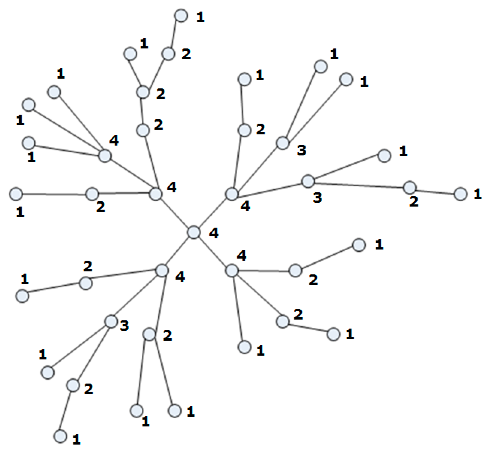
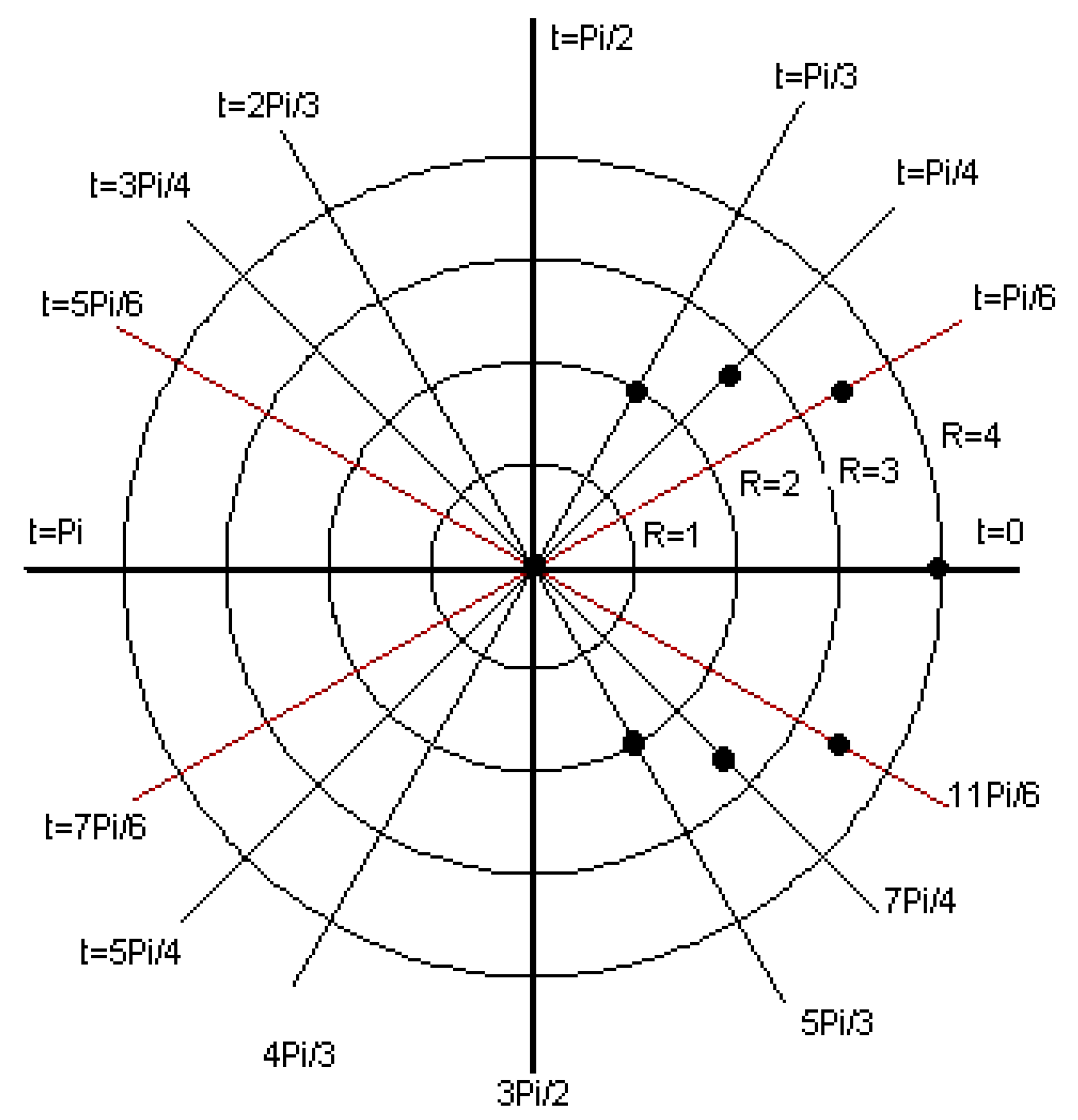
The property of self-similarity for a network means that the degree of distribution is invariant under renormalization, i.e., a network is self-similar if it satisfies P(k)~k−y for an appropriate renormalization procedure. The fractality of a network (also called fractal scaling or topological fractality) infers a power-law relationship between the minimum number of boxes needed to cover the entire network and the size of the boxes, i.e., a network is fractal if the box dimension D exists. However, some networks are self-similar but not fractal. Typical examples of such networks are the Internet and hierarchical graph sequence models. Thus, self-similarity and fractality do not always imply each other for complex networks [23,24,25,26]. Figure 1, Figure 2 and Figure 3 demonstrate our approach and analysis.
First of all, all fixed nodes of the network are presented in the Cartesian coordinate system (step 1). Fixed nodes present a location on the map. If a logistic network is not optimizing, we use a method for optimization. We weight all nodes by the number w of edges that each node has.
We then transform the nodes of the graph into a polar coordinate system (step 2). This means that all nodes have two coordinates (r,φ).
For all ri, we see how many of the nodes are on the circle with radius i. We calculate ni, which represents the number of nodes in the polar coordinate system with the circle with radius i as (3):
where represents the number of nodes. All nodes Ti(ri, ni) represent all points from the graph network in the polar coordinate system, which is a linear graph Γ(r, n). In addition, the linear graph Γ(r, n) presents points T1(r1, n1), T2(r2, n2) … Tk(rk, nk).
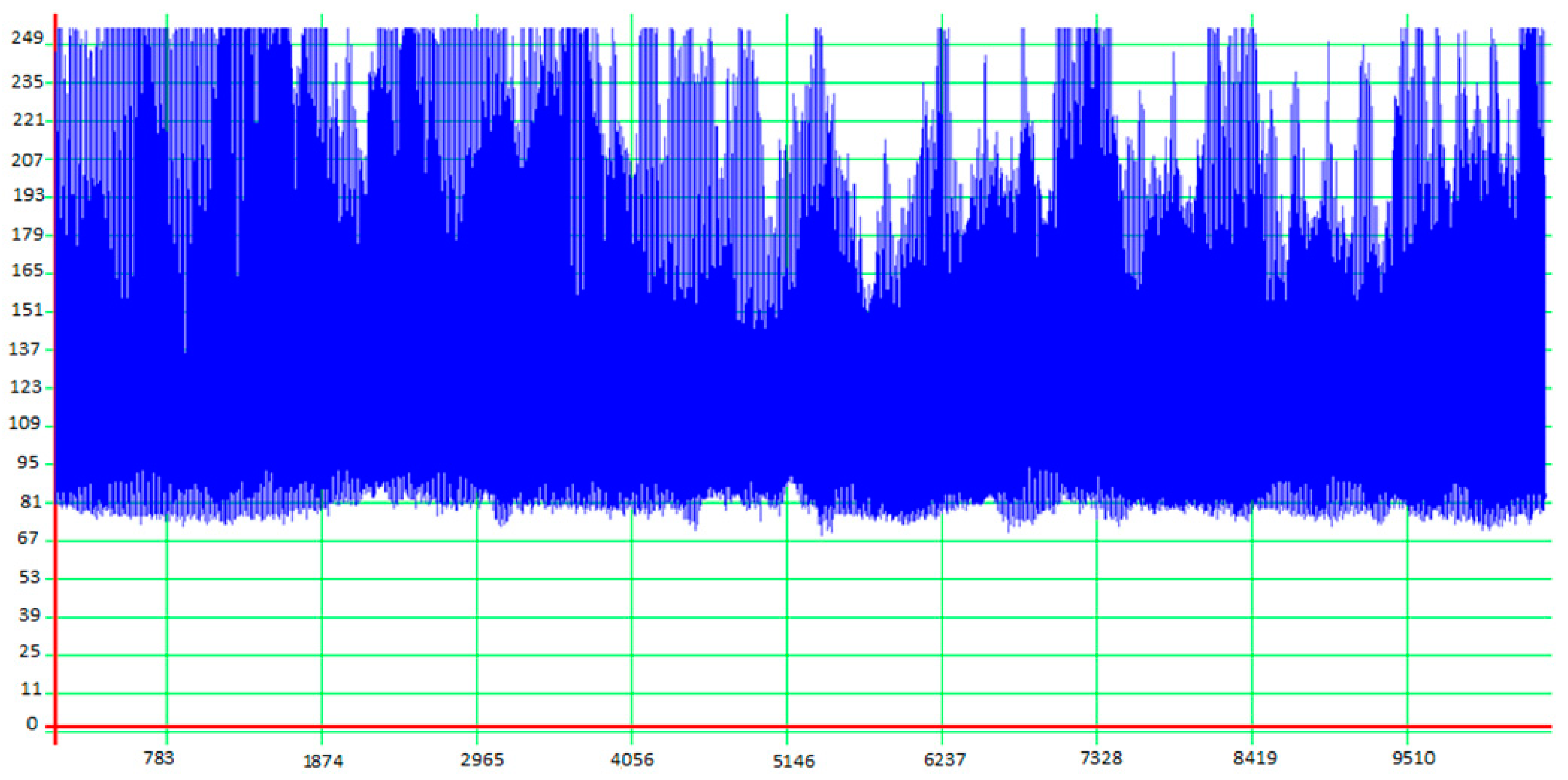
For this graph, we estimate the Hurst exponent H [23] (step 3).
After this, we can calculate the fractal dimension with equation D = 2–H. The Hurst exponent H ∈ (0, 1); thus, the fractal dimension of complex networks is D ∈ (1, 2).
Fractal and self-similarity properties of complex networks have attracted much attention because a variety of real, complex networks exhibit the property of self-similarity. This work aimed to study network science from a mathematical point of view, especially concerning the connection between networks and fractals. Complex networks have attracted increasing interest in various fields of science since they can be used to describe the structure and physical properties of many real complex systems. We presented a way of mathematically modeling complex networks with fractals. Prompted by the observation of the self-similar nature of several real networks, we described a new method. This was adapted from the study of fractals to investigate networks.
4. Bus Transport System
A transportation system is described as the collection of elements and their interactions that result in a demand for travel within a certain region and a supply of transportation services to meet that need. The municipality of Novo mesto is one of the largest Slovenian municipalities in terms of population. According to the Statistical Office of Slovenia, in 2019 it had a population of just over 24,000 The population density was 157 people per square kilometer, which means that the population density is higher than the national average of 103 inhabitants per km2. The municipality measures 236 km2. Novo mesto is the urban center of the Municipality of Novo mesto. It is also the administrative, educational, health, economic, and cultural center of the wider region of Southeastern Slovenia. With its industry, Novo mesto is the carrier of the fastest economic development in the region. A strong automotive, pharmaceutical, and cosmetic industry, and the insulation materials industry (Krka, Revoz, Adria Mobil, TPV) have developed, which also attracts labor from elsewhere. Maribor is the second-largest city in Slovenia and has a population of 95,000. Maribor has a developed public transport system. Celje is the third-largest city in Slovenia, with a population of 38,000, and has a developed public transport system. The city of Nova Gorica is the ninth-largest city of Slovenia, with a population of 13,000, and has a developed public transport system.
5. Data Mining
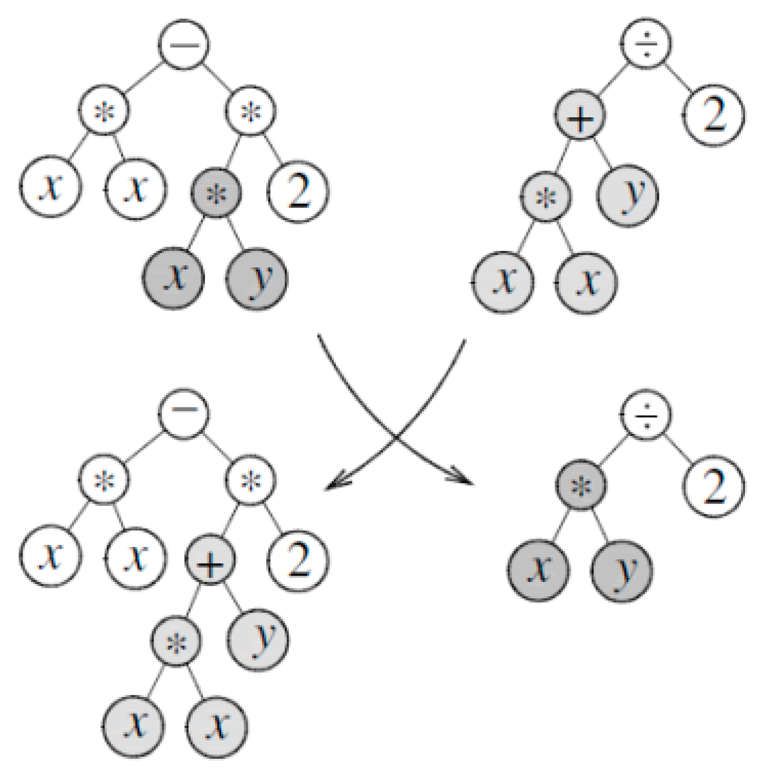
For predicting the complexity of bus transport systems, we use the method of an intelligent system, i.e., genetic programming, linear regression, and neural network. Genetic programming (GP) is an algorithm from the family of evolutionary algorithms. In nature, evolution has proven to be a very successful system for the further development and optimization of all living beings. Evolutionary algorithms use simple models to simulate the essential successful features of the natural evolutionary process. They enable good solutions to be found with relatively little effort, even in the case of problems with a large search area. Data structures and algorithms are generated and optimized by evolutionary algorithms to solve given problems. This introduction to the GP is based on Koza [27], who described GP for the first time. The individuals that are evolutionarily developed during the GP are programs. The choice of the functions used within a genetic program depends on the respective area of application. An essential requirement for the selection of the functions that are made available to the genetic program is that a solution for the application problem can be put together from them. The genetic operators are the tools available to the evolutionary algorithm to improve the fitness of the population in the course of evolution. The most commonly used operators are crossover, mutation, and reproduction. Figure 4 presents the GP operation. We have different operation multiplication (*), division (/), addition (+), subtraction (−) with numbers (2) and parameters (x, y).
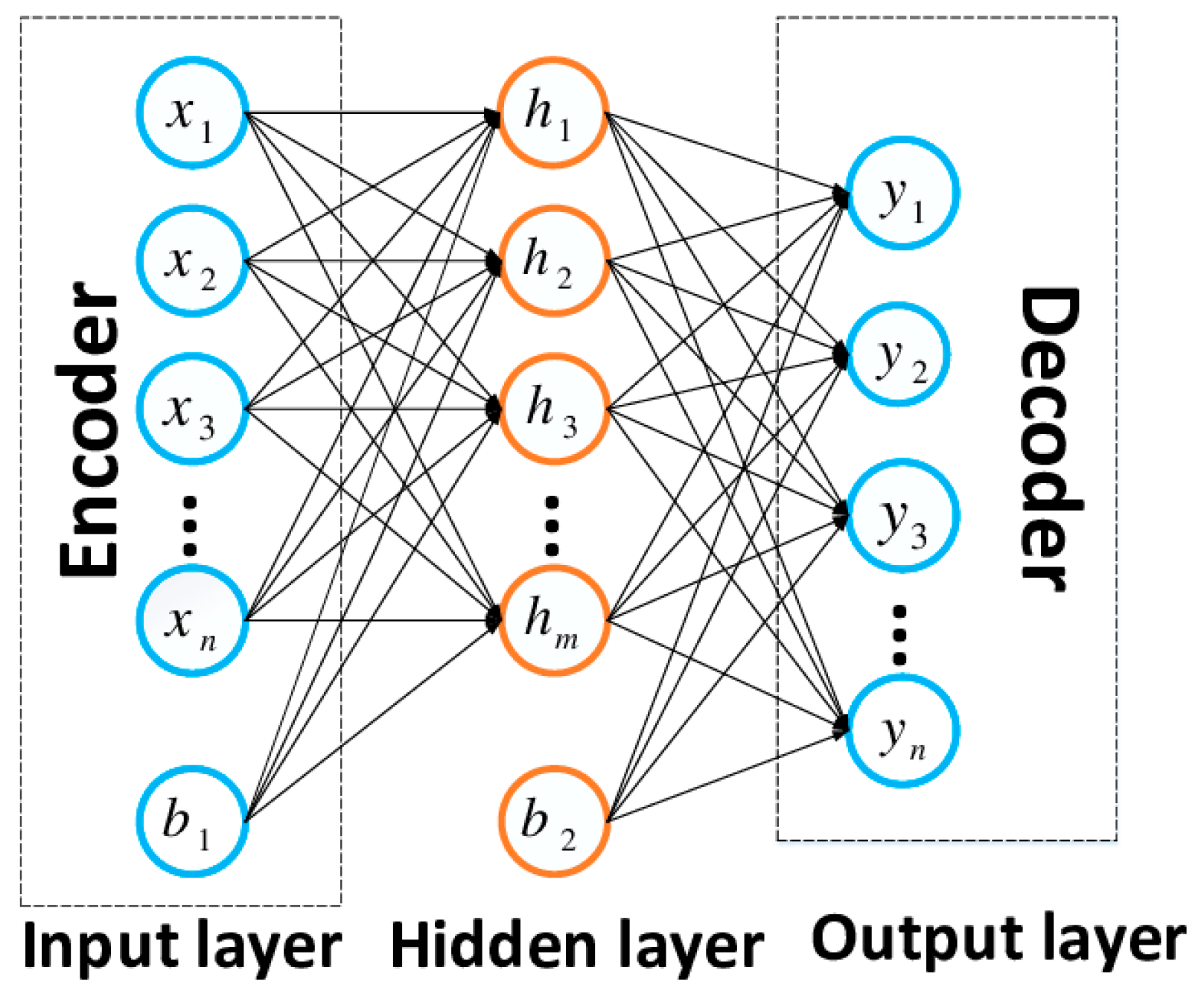
Artificial neural networks (ANN) [28] are inspired by the human brain and can be used for machine learning and artificial intelligence. Various problems can be solved via computer with these networks. The ANN is modeled to a certain extent on the structure of the biological brain. It consists of an abstract model of interconnected neurons, the special arrangement, and the connection of which can be used to solve computer-based application problems from various areas, such as statistics, technology, or economics. The neural network is a research subject in neuroinformatics and a branch of artificial intelligence. Neural networks have to be trained before they can solve problems. The structure and functioning of a neural network can be described in a greatly simplified manner as follows: The abstract model of a neural network consists of neurons, also called units or nodes. They can take in information from outside or other neurons and pass it on in modified form to other neurons or output it as a final result. A basic distinction can be made between input neurons, hidden neurons, and output neurons. The input neurons receive information in the form of patterns or signals from the outside world. The hidden neurons are located between the input and output neurons and represent internal information patterns. Output neurons pass information and signals on to the outside world as a result. The different neurons are connected via what are known as edges. This means that the output of one neuron can become the input of the next neuron. Depending on the strength and importance of the connection, the edge has a certain weighting. The stronger the weighting, the greater the influence a neuron can exert on another neuron via the connection. Figure 5 presents Artificial neural network (ANN). X present input data, h present hidden layer in an artificial neural network and is a layer in between input layers and output layers, y present output layer, which is result of prediction, b on is one of elements in input and hidden layer.
6. Results and Discussion
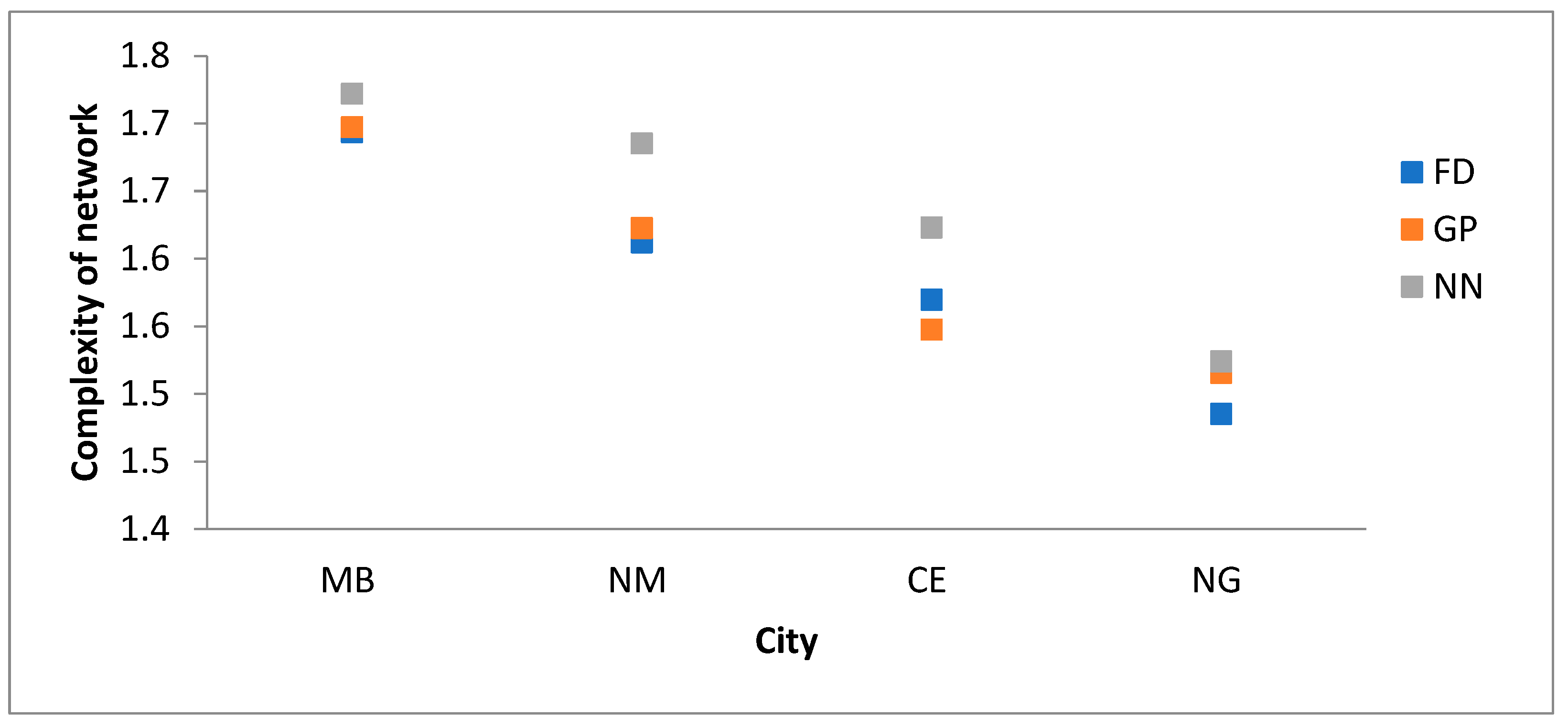
We use a new method of quantifying the complexity of fractal networks in the city of four cities in Slovenia, the center of network stations in the main bus station. We use the method of an intelligent system to predict the complexity of the bus stations network regarding the number of passengers, the population, stations, and lines. The bus transport network system (BTNS) in the city of Novo mesto (NM) is used by 300,000 passengers per year. The BTNS in NM has 94 stations and 7 lines. The complexity of the bus transport network is 1.6121. The bus transport network system (BTNS) in the city of Maribor (MB) is used by 4,000,000 passengers per year. The BTNS in MB has 200 stations and 23 lines. The complexity of the bus transport network is 1.6936.
The bus transport network system (BTNS) in the city of Celje (CE) is used by 150,000 passengers per year. The BTNS in CE has 35 stations and 6 lines. The complexity of the bus transport network is 1.5697. The bus transport network system (BTNS) in the city of Celje (NG) is used by 500,000 passengers per year. The BTNS in NG has 45 stations and 5 lines. The complexity of the bus transport network is 1.4951. Figure 6 represents the calculated and predicted complexity of the network. Equation (4) represents the genetic programming model (GP). We insert the number of PASSENGERS, POPULATION, STATIONS and LINE. The GP model gives us FD—COMPLEXITY of network. Table 1 present parameters for modeling complexity of bus transport network. Table 2 presents calculated and predicted complexity of the network.
MODEL OF GP:
FD = (2.945962 × (−0.1461 × PA + 14.87598 × PO) × (PO + (5.89124 × PO × (−0.1461 × PA + 14.87598 × PO))/((PO − (3.53816 × PO)/(PO + (5.389125 × PA × (−1315.261 + 88.4151 × L − 0.1461 × PO))/((PO + 24.2237/(6.84642 − 0.1683 × PA × PO − 14.8759 × PO × PO)) × S))) × S)))/(S × (PO + (2.94562 × (−0.1461 × PA + 14.87598 × PO))/(2 × L + (2.94562 × PO × (0.1461 + (12.7032 − L) × PO))/((8.9325 + L + PA−PO) × (L + S)))))
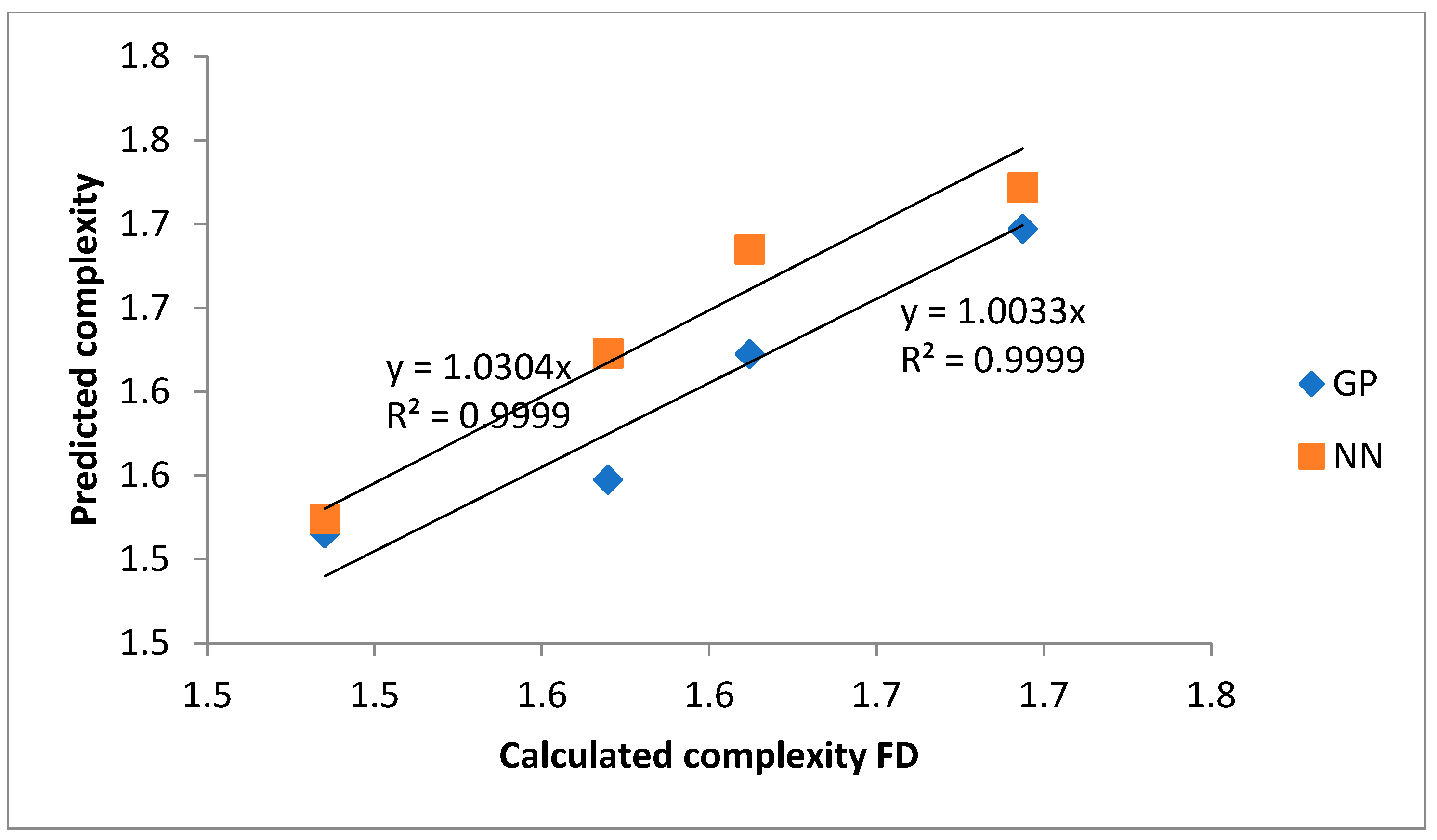
Correlation analysis is concerned with the degree of relationship between two variables, x, and y. We first assume that both x and y are quantitative, such as height and weight. Suppose a pair of values (x, y) is measured for each of the n objects in the sample. We can mark a point corresponding to a pair of magnitudes of each object on a 2D scatter plot. Typically, on a graph, x is placed on the horizontal axis and y is placed on the vertical axis. By placing points for all n objects, one obtains a scatter plot that tells the relationship between these two variables. Model adequacy analysis is an important step in modeling. To test the adequacy of multiple regression models, as well as paired linear regression, the coefficient of determination and its modifications are used, reflecting the features of the multiple model, as well as the procedures for testing statistical hypotheses and constructing confidence intervals for parameter estimates and forecasts of the dependent variable. It is the case, for instance, of the values of complexity, where those coefficients of determination are R2 = 0.9474 or R2 = 0.9277, depending on the specific ML methods used (GP and NN, respectively). The correspondence between the coefficients suggests that the two forecasting techniques are similarly effective. The coefficient of determination increases (more precisely, it almost always increases) as the number of regressors in the model increases. This leads to the fact that if, when assessing the quality of the model, one is guided by the usual coefficient R2, then equations with a large number of regressors will give a better result than with a smaller one. This can lead to the unjustified inclusion of a large number of insignificant regressors in the model. The inclusion of each additional regressor results in the loss of one degree of freedom. Figure 7 represents a graphical representation of data with the correlation of determination. It is the case of FD (Complexity) with coefficients.
An x and y relationship is linear if a straight line drawn through the central part of a cluster of points gives the best approximation of the observed relationship. It is possible to measure how close observations are to a straight line that best describes their linear relationship by calculating the Pearson correlation coefficient, commonly referred to simply as the correlation coefficient. Its true value in the population (general correlation coefficient) (Greek letter “rho” ρ) is estimated in the sample as r (sample correlation coefficient), which is usually obtained in the results of a computer calculation. Pearson coefficient ρGP = 0.9997 and ρNN = 0.7387.
7. Conclusions
The geometrization of networks, which enables us to view computer phenomena using the tools of graph theory and topology, has left a lasting impression in many areas including social networking, materials science, physics, and biomedical image processing. We have presented a new method for quantifying the complexity of a network. The combination of the methodologies utilized in this paper provides new insights into the concept of dimensionality in complex networks. In conclusion, we have shown that all networks with fixed nodes, which are presentable in 2D space, have complexity 1~D~2. The study of the relationship between network and fractal properties can be used in technology and medicine. This construction method may, then, also be of significance for the design of different networks and their topological characteristics. This connection between geometry, topology, and network behavior is fascinating and is of potential relevance to the new geometric approach introduced here.
Author Contributions
M.B.: Conceptualization, methodology, validation, writing—original draft preparation, and writing—review and editing; M.K., B.Š., M.C. and D.M.: review and editing. All authors have read and agreed to the published version of the manuscript.
Funding
This project was supported by the Republic of Slovenia and the European Union under the European Regional Development Fund (grant “Raziskovalci-2.1-FIŠ-952001”, implementation of the operation no. C3330-19-952001). This paper belongs to a research path funded by University of Catania (Starting Grant 2020–2022 Linea 3—Progetto NASCAR—Prot. 308811).
Institutional Review Board Statement
Not applicable.
Informed Consent Statement
Not applicable.
Data Availability Statement
Not applicable.
Conflicts of Interest
The authors declare no conflict of interest.
References
- Song, C.; Havlin, S.; Makse, H.A. Self-similarity of complex networks. Nature 2005, 433, 392–395. [Google Scholar] [CrossRef] [PubMed] [Green Version]
- Mandelbrot, B.B. The Fractal Geometry of Nature; W.H. Freeman: New York, NY, USA, 1982. [Google Scholar]
- Willinger, W.; Paxson, V.; Riedi, R.H.; Taqqu, M.S. Theory and Applications of Long-Range Dependence; Doukhan, P., Oppenheim, G., Taqqu, M.S., Eds.; Birkhäuser: Boston, MA, USA, 2003; pp. 373–407. [Google Scholar]
- Qian, B.; Rasheed, K. Hurst exponent and financial market predictability. In Proceedings of the 2nd IASTED International Conference on Financial Engineering and Applications, Cambridge, MA, USA, 8–10 November 2004; pp. 203–209. [Google Scholar]
- Erdős, P.; Rényi, A. On the evolution of random graphs. Magyar Tud. Akad. Mat. Kutató Int. Közl 1960, 5, 17–61. [Google Scholar]
- Bollobás, B.E.; Riordan, O.; Spencer, J.; Tusnády, G. The degree sequence of a scale-free random graph process. Random Struct. Algorithms 2001, 18, 279–290. [Google Scholar] [CrossRef] [Green Version]
- Barabási, A.L.; Albert, R. Emergence of scaling in random networks. Science 1999, 286, 509–512. [Google Scholar] [CrossRef] [Green Version]
- Abrahao, B.; Chierichetti, F.; Kleinberg, R.; Panconesi, A. Trace complexity of network inference. In Proceedings of the 19th ACM SIGKDD International Conference on Knowledge Discovery and Data Mining, Chicago, IL, USA, 11–14 August 2013; pp. 491–499. [Google Scholar]
- Feder, J. Fractals; Plenum: New York, NY, USA, 1988. [Google Scholar]
- Csányi, G.; Szendrői, B. Fractal–small-world dichotomy in real-world networks. Phys. Rev. 2004, 70, 16122. [Google Scholar] [CrossRef] [Green Version]
- Gastner, M.T.; Newman, M.E. The spatial structure of networks. Eur. Phys. J. B Condens. Matter Complex Syst. 2006, 49, 247–252. [Google Scholar] [CrossRef] [Green Version]
- Song, C.; Havlin, S.; Makse, H.A. Origins of Fractality in the Growth of Complex Networks. Nat. Phys. 2006, 2, 275–281. [Google Scholar] [CrossRef] [Green Version]
- Kim, J.S.; Goh, K.-I.; Salvi, G.; Oh, E.; Kahngand, B.; Kim, D. Fractality in complex networks: Critical and supercritical skeletons. Phys. Rev. E. 2007, 75, 16110. [Google Scholar] [CrossRef] [Green Version]
- Shao, J.; Buldyrev, S.V.; Cohen, R.; Kitsak, M.; Havlin, S.; Stanley, H.E. Fractal boundaries of complex networks. Europhys. Lett. 2007, 84, 48004. [Google Scholar] [CrossRef] [Green Version]
- Li, B.-G.; Yu, Z.-G.; Zhou, Y. Fractal and multifractal properties of a family of fractal networks. J. Stat. Mech. Theory Exp. 2014, 2, P02020. [Google Scholar] [CrossRef] [Green Version]
- Gallos, K.L.; Makse, A.H.; Sigman, M. A small world of weak ties provides optimal global integration of self-similar modules in functional brain networks. Proc. Natl. Acad. Sci. USA 2012, 109, 2825–2830. [Google Scholar] [CrossRef] [PubMed] [Green Version]
- Shanker, O. Graph zeta function and dimension of complex network. Mod. Phys. Lett. B. 2007, 21, 639–644. [Google Scholar] [CrossRef]
- Gao, L.; Hu., Y.; Di, Z. Accuracy of the ball-covering approach for fractal dimensions of complex networks and a rank-driven algorithm. Phys. Rev. E. 2008, 78, 46109. [Google Scholar] [CrossRef] [PubMed]
- Daqing, L.; Kosmidis, K.; Bunde, A.; Havlin, S. Dimension of spatially embedded networks. Nat. Phys. 2011, 7, 481–484. [Google Scholar] [CrossRef] [Green Version]
- Lee, C.; Jung, S. Statistical self-similar properties of complex networks. Phys. Rev. E. 2006, 73, 66102. [Google Scholar] [CrossRef] [Green Version]
- Yook, S.-H.; Jeong, H.; Barabási, A.-L. Modeling the Internet’s large-scale topology. Proc. Natl. Acad. Sci. USA 2002, 99, 13382–13386. [Google Scholar] [CrossRef] [Green Version]
- Sun, W.; Liu, S. Consensus of Julia Sets. Fractal Fract. 2022, 6, 43. [Google Scholar] [CrossRef]
- Corrêa, E.A.; Lopes, A.A.; Amancio, D.R. Word sense disambiguation: A complex network approach. Inf. Sci. 2018, 442–443, 103–113. [Google Scholar] [CrossRef] [Green Version]
- da Mata, A.S. Complex Networks: A Mini-Review. Braz. J. Phys. 2020, 50, 658–672. [Google Scholar] [CrossRef]
- Liu, J.; Li, J.; Chen, Y.; Chen, X.; Zhou, Z.; Yang, Z.; Zhang, C.-J. Modeling complex networks with accelerating growth and aging effect. Phys. Lett. A 2019, 383, 1396–1400. [Google Scholar] [CrossRef]
- Song, W.; Sheng, W.; Li, D.; Wu, C.; Ma, J. Modeling Complex Networks Based on Deep Reinforcement Learning. Front. Phys. 2022, 9, 822581. [Google Scholar] [CrossRef]
- Koza, J.R. Genetic Programming: A Paradigm for Genetically Breeding Populations of Computer Programs to Solve Problems; Technical Report STAN-CS-90-1314; University Computer Science Department Technical Report: Stanford, CA, USA, 1990. [Google Scholar]
- Gessler, J. Sensor for food analysis applying impedance spectroscopy and artificial neural networks. RiuNet UPV 2021, 1, 8–12. [Google Scholar]
Figure 1.
Step 1. Network with different weight (1–4).

Figure 2.
Step 2.

Figure 3.
Step 3.

Figure 4.
Genetic programming (GP) operation.

Figure 5.
Artificial neural networks (ANN).

Figure 6.
Calculated and predicted complexity of the network.

Figure 7.
A graphical representation of data with the correlation of determination. It is the case of FD (Complexity) with coefficients.
Figure 7.
A graphical representation of data with the correlation of determination. It is the case of FD (Complexity) with coefficients.


Table 1.
Parameters for modeling complexity of bus transport network.
| City | # Passengers (PA) | # Population (PO) | # Stations (S) | # Line (L) | FD—Complexity |
|---|---|---|---|---|---|
| MB | 4,000,000 | 95,000 | 200 | 23 | 1.6936 |
| NM | 300,000 | 24,000 | 94 | 7 | 1.6121 |
| CE | 150,000 | 38,000 | 35 | 6 | 1.5697 |
| NG | 500,000 | 13,000 | 45 | 5 | 1.4951 |
Table 2.
Calculated and predicted complexity of the network.
| FD | GP | NN |
|---|---|---|
| 1.6936 | 1.6973 | 1.722 |
| 1.6121 | 1.6126 | 1.6852 |
| 1.5697 | 1.5476 | 1.6231 |
| 1.4951 | 1.4956 | 1.5241 |
Publisher’s Note: MDPI stays neutral with regard to jurisdictional claims in published maps and institutional affiliations. |
© 2022 by the authors. Licensee MDPI, Basel, Switzerland. This article is an open access article distributed under the terms and conditions of the Creative Commons Attribution (CC BY) license (https://creativecommons.org/licenses/by/4.0/).
Share and Cite
MDPI and ACS Style
Babič, M.; Marinković, D.; Kovačič, M.; Šter, B.; Calì, M. A New Method of Quantifying the Complexity of Fractal Networks. Fractal Fract. 2022, 6, 282. https://doi.org/10.3390/fractalfract6060282
AMA Style
Babič M, Marinković D, Kovačič M, Šter B, Calì M. A New Method of Quantifying the Complexity of Fractal Networks. Fractal and Fractional. 2022; 6(6):282. https://doi.org/10.3390/fractalfract6060282
Chicago/Turabian StyleBabič, Matej, Dragan Marinković, Miha Kovačič, Branko Šter, and Michele Calì. 2022. "A New Method of Quantifying the Complexity of Fractal Networks" Fractal and Fractional 6, no. 6: 282. https://doi.org/10.3390/fractalfract6060282